
Interfaces for Explaining Transformer Language Models
Interfaces for exploring transformer language models by looking at input saliency and neuron activation.
Tap or hover over the output tokens:
Explorable #2: Neuron activation analysis reveals four groups of neurons, each is associated with generating a certain type of token
Tap or hover over the sparklines on the left to isolate a certain factor:
The Transformer architecture has been powering a number of the recent advances in NLP. A breakdown of this architecture is provided here . Pre-trained language models based on the architecture, in both its auto-regressive (models that use their own output as input to next time-steps and that process tokens from left-to-right, like GPT2) and denoising (models trained by corrupting/masking the input and that process tokens bidirectionally, like BERT) variants continue to push the envelope in various tasks in NLP and, more recently, in computer vision. Our understanding of why these models work so well, however, still lags behind these developments.
This exposition series continues the pursuit to interpret and visualize the inner-workings of transformer-based language models. We illustrate how some key interpretability methods apply to transformer-based language models. This article focuses on auto-regressive models, but these methods are applicable to other architectures and tasks as well.
This is the first article in the series. In it, we present explorables and visualizations aiding the intuition of:
- Input Saliency methods that score input tokens importance to generating a token.
- Neuron Activations and how individual and groups of model neurons spike in response to inputs and to produce outputs.
The next article addresses Hidden State Evolution across the layers of the model and what it may tell us about each layer's role.
In the language of Interpretable Machine Learning (IML) literature like Molnar et al., input saliency is a method that explains individual predictions. The latter two methods fall under the umbrella of "analyzing components of more complex models", and are better described as increasing the transparency of transformer models.
Moreover, this article is accompanied by reproducible notebooks and Ecco - an open source library to create similar interactive interfaces directly in Jupyter notebooks for GPT-based models from the HuggingFace transformers library.
If we're to impose the three components we're examining to explore the architecture of the transformer, it would look like the following figure.
By introducing tools that visualize input saliency, the evolution of hidden states, and neuron activations, we aim to enable researchers to build more intuition about Transformer language models.
Input Saliency
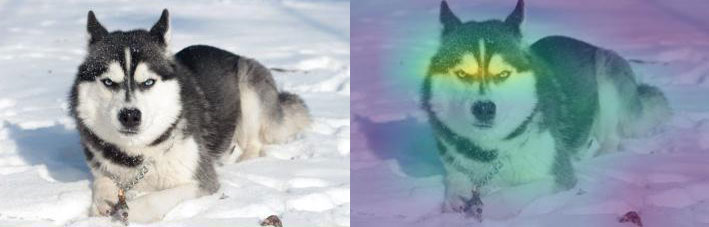
When a computer vision model classifies a picture as containing a husky, saliency maps can tell us whether the classification was made due to the visual properties of the animal itself, or because of the snow in the background. This is a method of attribution explaining the relationship between a model's output and inputs -- helping us detect errors and biases, and better understand the behavior of the system.
Multiple methods exist for assigning importance scores to the inputs of an NLP model. The literature is most often concerned with this application for classification tasks, rather than natural language generation. This article focuses on language generation. Our first interface calculates feature importance after each token is generated, and by hovering or tapping on an output token, imposes a saliency map on the tokens responsible for generating it.
The first example for this interface asks GPT2-XL for William Shakespeare's date of birth. The model is correctly able to produce the date (1564, but broken into two tokens: " 15" and "64", because the model's vocabulary does not include " 1564" as a single token). The interface shows the importance of each input token when generating each output token:
GPT2-XL is able to tell the birth date of William Shakespeare expressed in two tokens. In generating the first token, 53% of the importance is assigned to the name (20% to the first name, 33% to the last name). The next most important two tokens are " year" (22%) and " born" (14%). In generating the second token to complete the date, the name still is the most important with 60% importance, followed by the first portion of the date -- a model output, but an input to the second time step.
This prompt aims to probe world knowledge. It was generated using greedy decoding. Smaller variants of GPT2 were not able to output the correct date.
Our second example attempts to both probe a model's world knowledge, as well as to see if the model repeats the patterns in the text (simple patterns like the periods after numbers and like new lines, and slightly more involved patterns like completing a numbered list). The model used here is DistilGPT2.
This explorable shows a more detailed view that displays the attribution percentage for each token -- in case you need that precision.
Tap or hover over the output tokens.
This was generated by DistilGPT2 and attribution via Gradients X Inputs. Output sequence is cherry-picked to only include European countries and uses sampled (non-greedy) decoding. Some model runs would include China, Mexico, and other countries in the list. With the exception of the repeated " Finland", the model continues the list alphabetically.
Another example that we use illustratively in the rest of this article is one where we ask the model to complete a simple pattern:
Every generated token ascribes the first token in the input the highest feature importance score. Then throughout the sequence, the preceding token, and the first three tokens in the sequence are often the most important. This uses Gradient × Inputs on GPT2-XL.
This prompt aims to probe the model's response to syntax and token patterns. Later in the article, we build on it by switching to counting instead of repeating the digit ' 1'. Completion gained using greedy decoding. DistilGPT2 is able to complete it correctly as well.
It is also possible to use the interface to analyze the responses of a transformer-based conversational agent. In the following example, we pose an existential question to DiabloGPT:
Tap or hover over the output tokens.
This was the model's first response to the prompt. The question mark is attributed the highest score in the beginning of the output sequence. Generating the tokens " will" and " ever" assigns noticeably more importance to the word " ultimate". This uses Gradient × Inputs on DiabloGPT-large.
![]()
About Gradient-Based Saliency
Demonstrated above is scoring feature importance based on Gradients X Inputs-- a gradient-based saliency method shown by Atanasova et al. to perform well across various datasets for text classification in transformer models.
To illustrate how that works, let's first recall how the model generates the output token in each time step. In the following figure, we see how ① the language model's final hidden state is projected into the model's vocabulary resulting in a numeric score for each token in the model's vocabulary. Passing that scores vector through a softmax operation results in a probability score for each token. ② We proceed to select a token (e.g. select the highest-probability scoring token, or sample from the top scoring tokens) based on that vector.
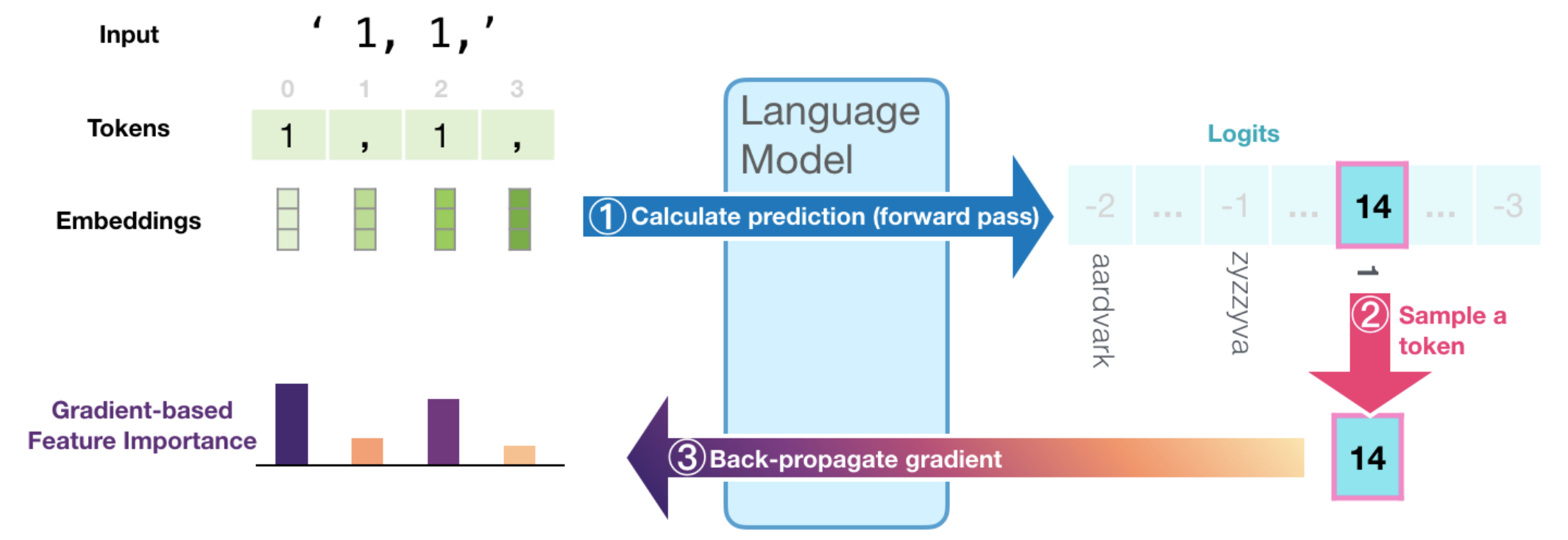
③ By calculating the gradient of the selected logit (before the softmax) with respect to the inputs by back-propagating it all the way back to the input tokens, we get a signal of how important each token was in the calculation resulting in this generated token. That assumption is based on the idea that the smallest change in the input token with the highest feature-importance value makes a large change in what the resulting output of the model would be.
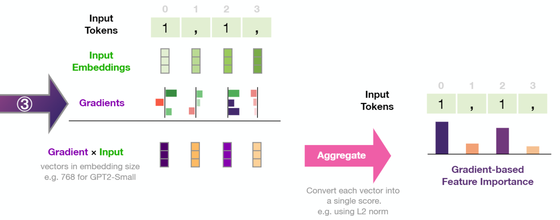
The resulting gradient vector per token is then multiplied by the input embedding of the respective token. Taking the L2 norm of the resulting vector results in the token's feature importance score. We then normalize the scores by dividing by the sum of these scores.
More formally, gradient × input is described as follows:
Where is the embedding vector of the input token at timestep i, and is the back-propagated gradient of the score of the selected token unpacked as follows:
- is the list of input token embedding vectors in the input sequence (of length )
- is the score of the selected token after a forward pass through the model (selected through any one of a number of methods including greedy/argmax decoding, sampling, or beam search). With the c standing for "class" given this is often described in the classification context. We're keeping the notation even though in our case, "token" is more fitting.
This formalization is the one stated by Bastings et al. except the gradient and input vectors are multiplied element-wise. The resulting vector is then aggregated into a score via calculating the L2 norm as this was empirically shown in Atanasova et al. to perform better than other methods (like averaging).
Neuron Activations
The Feed Forward Neural Network (FFNN) sublayer is one of the two major components inside a transformer block (in addition to self-attention). It accounts for 66% of the parameters of a transformer block and thus provides a significant portion of the model's representational capacity. Previous work has examined neuron firings inside deep neural networks in both the NLP and computer vision domains. In this section we apply that examination to transformer-based language models.
Continue Counting: 1, 2, 3, ___
To guide our neuron examination, let's present our model with the input "1, 2, 3" in hopes it would echo the comma/number alteration, yet also keep incrementing the numbers.
It succeeds.
By using the methods we'll discuss in Article #2 (following the lead of nostalgebraist), we can produce a graphic that exposes the probabilities of output tokens after each layer in the model. This looks at the hidden state after each layer, and displays the ranking of the ultimately produced output token in that layer.
For example, in the first step, the model produced the token " 4". The first column tells us about that process. The bottom most cell in that column shows that the token " 4" was ranked #1 in probability after the last layer. Meaning that the last layer (and thus the model) gave it the highest probability score. The cells above indicate the ranking of the token " 4" after each layer.
By looking at the hidden states, we observe that the model gathers confidence about the two patterns of the output sequence (the commas, and the ascending numbers) at different layers.
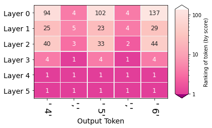
What happens at Layer 4 which makes the model elevate the digits (4, 5, 6) to the top of the probability distribution?
We can plot the activations of the neurons in layer 4 to get a sense of neuron activity. That is what the first of the following three figures shows.
It is difficult, however, to gain any interpretation from looking at activations during one forward pass through the model.
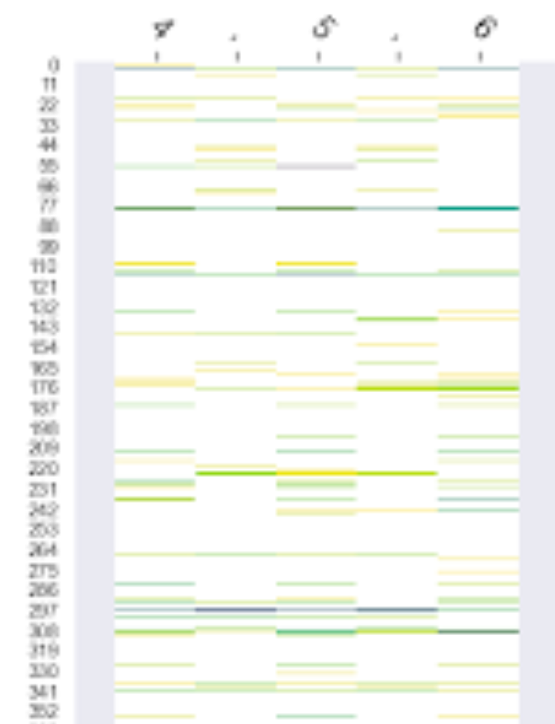
The figures below show neuron activations while five tokens are generated (' 4 , 5 , 6'). To get around the sparsity of the firings, we may wish to cluster the firings, which is what the subsequent figure shows.
|
Each row is a neuron. Only neurons with positive activation are colored. The darker they are, the more intense the firing. |
|
Each row corresponds to a neuron in the feedforward neural network of layer #4. Each column is that neuron's status when a token was generated (namely, the token at the top of the figure). A view of the first 400 neurons shows how sparse the activations usually are (out of the 3072 neurons in the FFNN layer in DistilGPT2). |
|
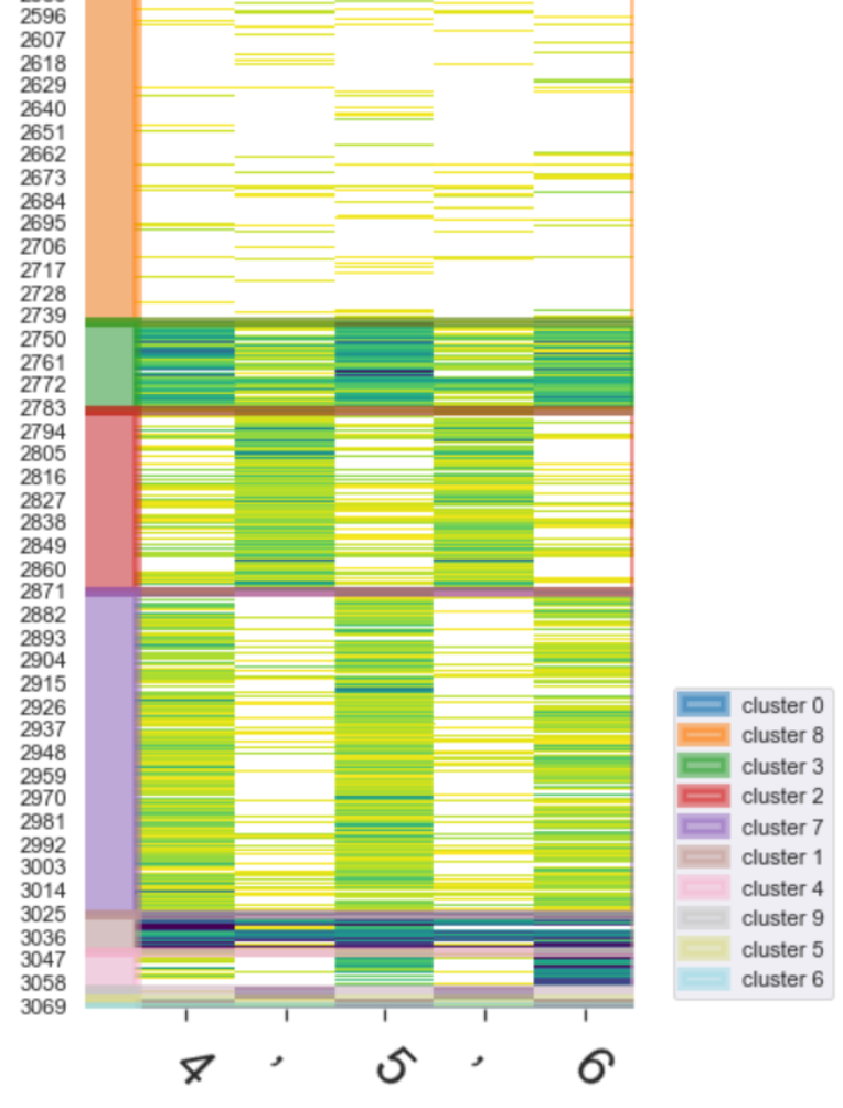
Clustering Neurons by Activation Values To locate the signal, the neurons are clustered (using kmeans on the activation values) to reveal the firing pattern. We notice:
|
If visualized and examined properly, neuron firings can reveal the complementary and compositional roles that can be played by individual neurons, and groups of neurons.
Even after clustering, looking directly at activations is a crude and noisy affair. As presented in Olah et al., we are better off reducing the dimensionality using a matrix decomposition method. We follow the authors' suggestion to use Non-negative Matrix Factorization (NMF) as a natural candidate for reducing the dimensionality into groups that are potentially individually more interpretable. Our first experiments were with Principal Component Analysis (PCA), but NMF is a better approach because it's difficult to interpret the negative values in a PCA component of neuron firings.
Factor Analysis
By first capturing the activations of the neurons in FFNN layers of the model, and then decomposing them into a more manageable number of factors (using) using NMF, we are able to shed light on how various neurons contributed towards each generated token.
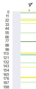
The simplest approach is to break down the activations into two factors. In our next interface, we have the model generate thirty tokens, decompose the activations into two factors, and highlight each token with the factor with the highest activation when that token was generated:
Tap or hover over the sparklines on the left to isolate a certain factor
Factor #1 contains the collection of neurons that light up to produce a number. It is a linear transformation of 5,449 neurons (30% of the 18,432 neurons in the FFNN layers: 3072 per layer, 6 layers in DistilGPT2).
Factor #2 contains the collection of neurons that light up to produce a comma. It is a linear transformation of 8,542 neurons (46% of the FFNN neurons).
The two factors have 4,365 neurons in common.
Note: The association between the color and the token is different in the case of the input tokens and output tokens. For the input tokens, this is how the neurons fired in response to the token as an input. For the output tokens, this is the activation value which produced the token. This is why the last input token and the first output token share the same activation value.
This interface is capable of compressing a lot of data that showcase the excitement levels of factors composed of groups of neurons. The sparklines on the left give a snapshot of the excitement level of each factor across the entire sequence. Interacting with the sparklines (by hovering with a mouse or tapping on touchscreens) displays the activation of the factor on the tokens in the sequence on the right.
We can see that decomposing activations into two factors resulted in factors that correspond with the alternating patterns we're analyzing (commas, and incremented numbers). We can increase the resolution of the factor analysis by increasing the number of factors. The following figure decomposes the same activations into five factors.
Tap or hover over the sparklines on the left to isolate a certain factor
- Decomposition into five factors shows the counting factor being broken down into three factors, each addressing a distinct portion of the sequence (start, middle, end).
- The yellow factor reliably tracks generating the commas in the sequence.
- The blue factor is common across various GPT2 factors -- it is of neurons that intently focus on the first token in the sequence, and only on that token.
We can start extending this to input sequences with more content, like the list of EU countries:
Tap or hover over the sparklines on the left to isolate a certain factor
Another example, of how DistilGPT2 reacts to XML, shows a clear distinction of factors attending to different components of the syntax. This time we are breaking down the activations into ten components:
Tap or hover over the sparklines on the left to isolate a certain factor
Factorizing neuron activations in response to XML (that was generated by an RNN from ) into ten factors results in factors corresponding to:
- New-lines
- Labels of tags, with higher activation on closing tags
- Indentation spaces
- The '<' (less-than) character starting XML tags
- The large factor focusing on the first token. Common to GPT2 models.
- Two factors tracking the '>' (greater than) character at the end of XML tags
- The text inside XML tags
- The '</' symbols indicating closing XML tag
Factorizing Activations of a Single Layer
This interface is a good companion for hidden state examinations which can highlight a specific layer of interest, and using this interface we can focus our analysis on that layer of interest. It is straight-forward to apply this method to specific layers of interest. Hidden-state evolution diagrams, for example, indicate that layer #0 does a lot of heavy lifting as it often tends to shortlist the tokens that make it to the top of the probability distribution. The following figure showcases ten factors applied to the activations of layer 0 in response to a passage by Fyodor Dostoyevsky:
Tap or hover over the sparklines on the left to isolate a certain factor
Ten Factors from the activations the neurons in Layer 0 in response to a passage from Notes from Underground by Dostoevsky.
- Factors that focus on specific portions of the text (beginning, middle, and end. This is interesting as the only signal the model gets about how these tokens are connected are the positional encodings. This indicates the neurons that are keeping track of the order of words. Further examination is required to assess whether these FFNN neurons directly respond to the time signal, or if they are responding to a specific trigger in the self-attention layer's transformation of the hidden state.
- Factors corresponding to linguistic features, for example, we can see factors for pronouns (he, him), auxiliary verbs (would, will), other verbs (introduce, prove -- notice the understandable misfiring at the 'suffer' token which is a partial token of 'sufferings', a noun), linking verbs (is, are, were), and a factor that favors nouns and their adjectives ("fatal rubbish", "vulgar folly").
- A factor corresponding to commas, a syntactic feature.
- The first-token factor
We can crank up the resolution by increasing the number of factors. Increasing this to eighteen factors starts to reveal factors that light up in response to adverbs, and other factors that light up in response to partial tokens. Increase the number of factors more and you'll start to identify factors that light up in response to specific words ("nothing" and "man" seem especially provocative to the layer).
About Activation Factor Analysis
The explorables above show the factors resulting from decomposing the matrix holding the activations values of FFNN neurons using Non-negative Matrix Factorization. The following figure sheds light on how that is done:
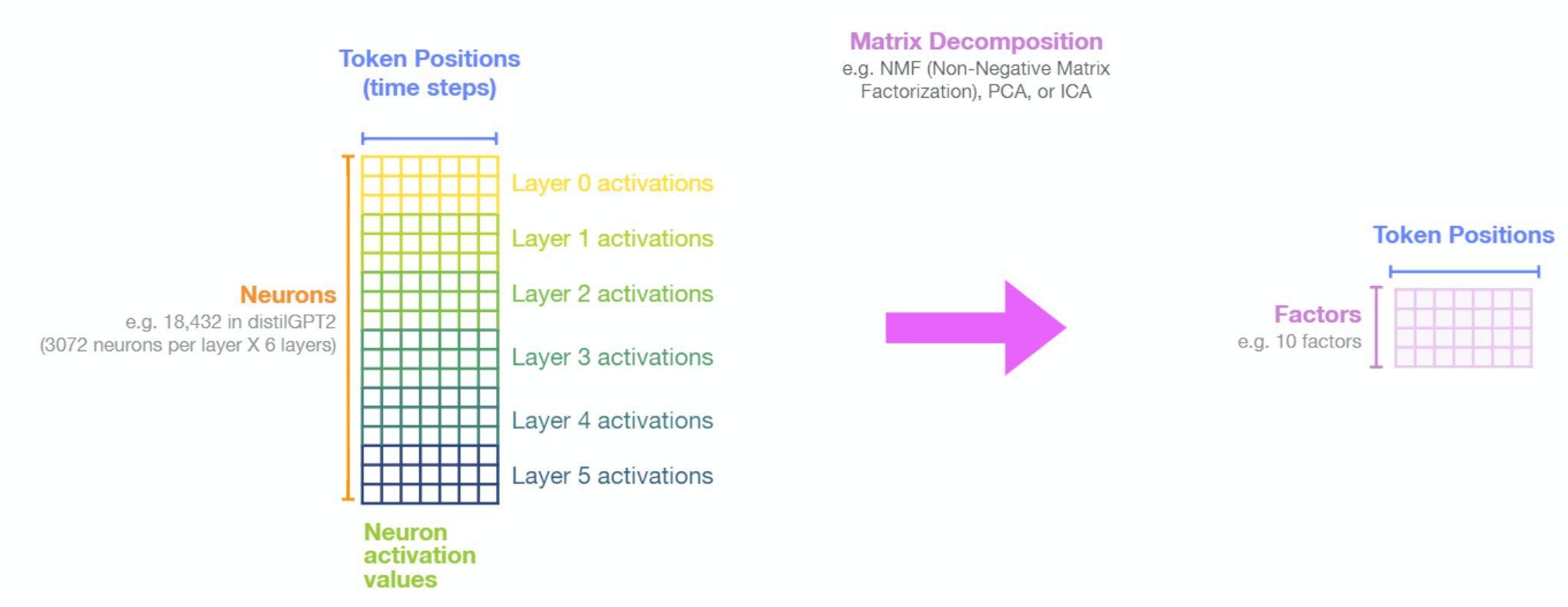
NMF reveals patterns of neuron activations inside one or a collection of layers.
Beyond dimensionality reduction, Non-negative Matrix Factorization can reveal underlying common behaviour of groups of neurons. It can be used to analyze the entire network, a single layer, or groups of layers.
![]()
Conclusion
This concludes the first article in the series. Be sure to click on the notebooks and play with Ecco! I would love your feedback on this article, series, and on Ecco in this thread. If you find interesting factors or neurons, feel free to post them there as well. I welcome all feedback!
Acknowledgements
This article was vastly improved thanks to feedback on earlier drafts provided by Abdullah Almaatouq, Ahmad Alwosheel, Anfal Alatawi, Christopher Olah, Fahd Alhazmi, Hadeel Al-Negheimish, Isabelle Augenstein, Jasmijn Bastings, Najla Alariefy, Najwa Alghamdi, Pepa Atanasova, and Sebastian Gehrmann.
References
Citation
Alammar, J. (2020). Interfaces for Explaining Transformer Language Models
[Blog post]. Retrieved from https://jalammar.github.io/explaining-transformers/
BibTex:
@misc{alammar2020explaining,
  title={Interfaces for Explaining Transformer Language Models},
  author={Alammar, J},
  year={2020},
  url={https://jalammar.github.io/explaining-transformers/}
}
