Here are eight observations I’ve shared recently on the Cohere blog and videos that go over them.:
Article: What’s the big deal with Generative AI? Is it the future or the present?
Article: AI is Eating The World
]]>And check out our How Transformer LLMs Work course!
]]>
Here are eight observations I’ve shared recently on the Cohere blog and videos that go over them.:
Article: What’s the big deal with Generative AI? Is it the future or the present?
Article: AI is Eating The World
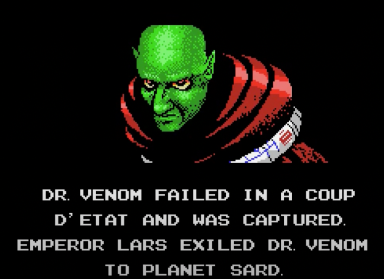
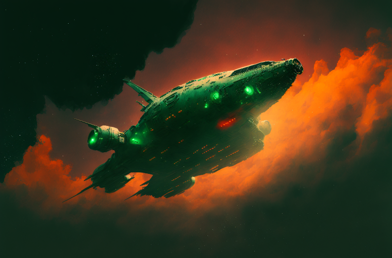
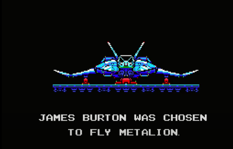
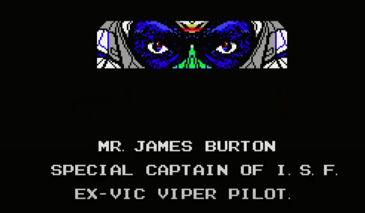
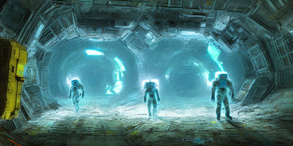
]]>Over the last few days, I used AI image generation to reproduce one of my childhood nightmares. I wrestled with Stable Diffusion, Dall-E and Midjourney to see how these commercial AI generation tools can help retell an old visual story - the intro cinematic to an old video game (Nemesis 2 on the MSX). This post describes the process and my experience in using these models/services to retell a story in higher fidelity graphics.
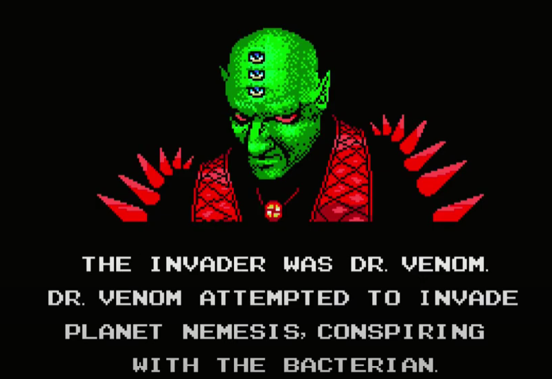
This fine-looking gentleman is the villain in a video game. Dr. Venom appears in the intro cinematic of Nemesis 2, a 1987 video game. This image, in particular, comes at a dramatic reveal in the cinematic.
Let’s update these graphics with visual generative AI tools and see how they compare and where each succeeds and fails.
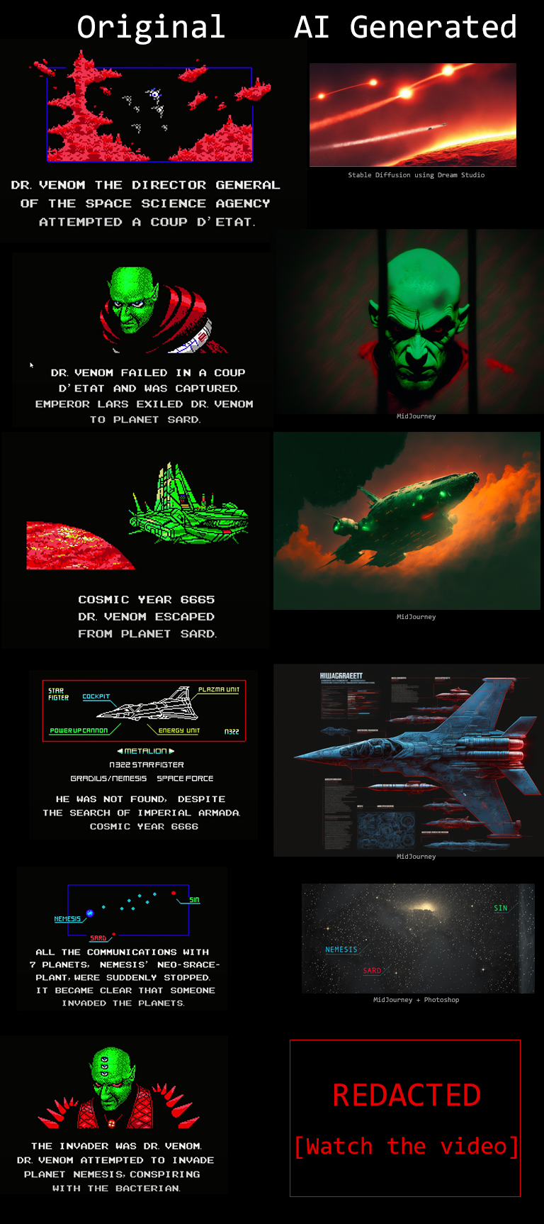
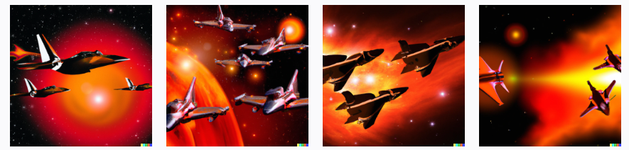
Here’s a side-by-side look at the panels from the original cinematic (left column) and the final ones generated by the AI tools (right column):
This figure does not show the final Dr. Venom graphic because I want you to witness it as I had, in the proper context and alongside the appropriate music. You can watch that here:
Original image
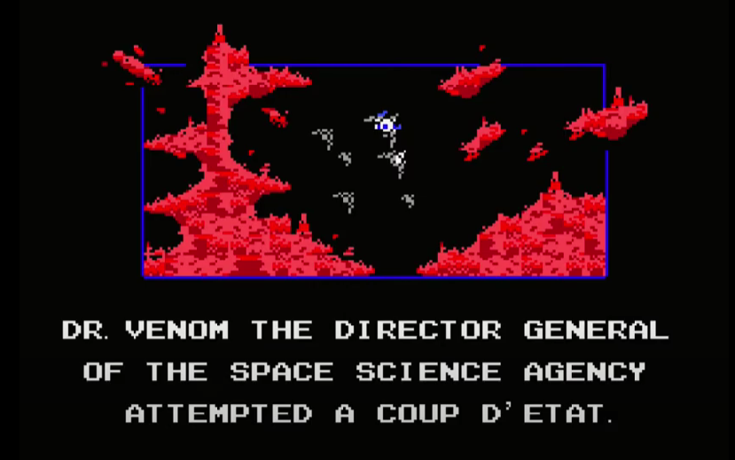
The final image was generated by Stable Diffusion using Dream Studio.

The road to this image, however, goes through generating over 30 images and tweaking prompts. The first kind of prompt I’d use is something like:
fighter jets flying over a red planet in space with stars in the black sky
This leads Dall-E to generate these candidates
Pasting a similar prompt into Dream Studio generates these candidates:
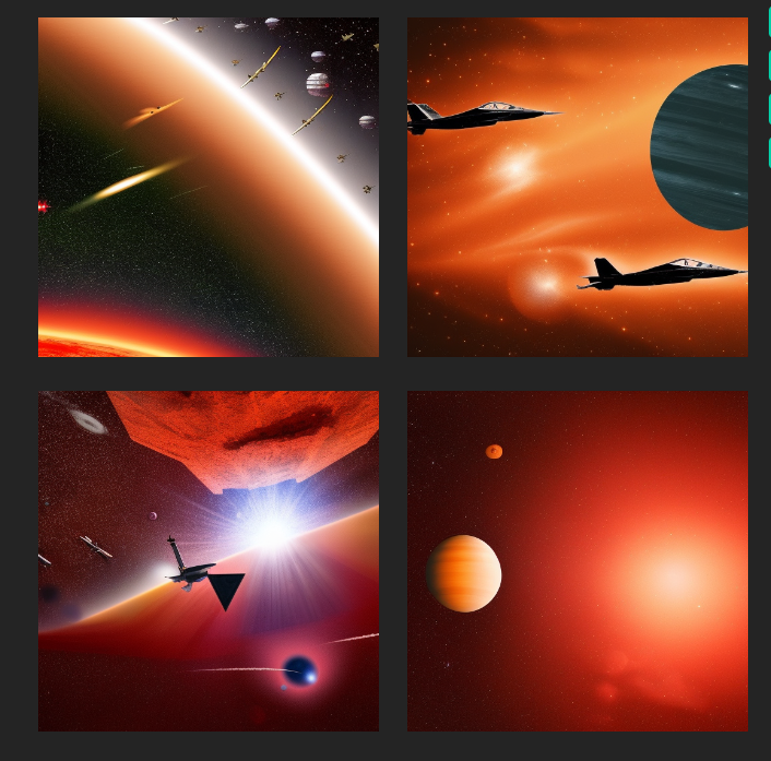
This showcases a reality of the current batch of image generation models. It is not enough for your prompt to describe the subject of the image. Your image creation prompt/spell needs to mention the exact arcane keywords that guide the model toward a specific style.
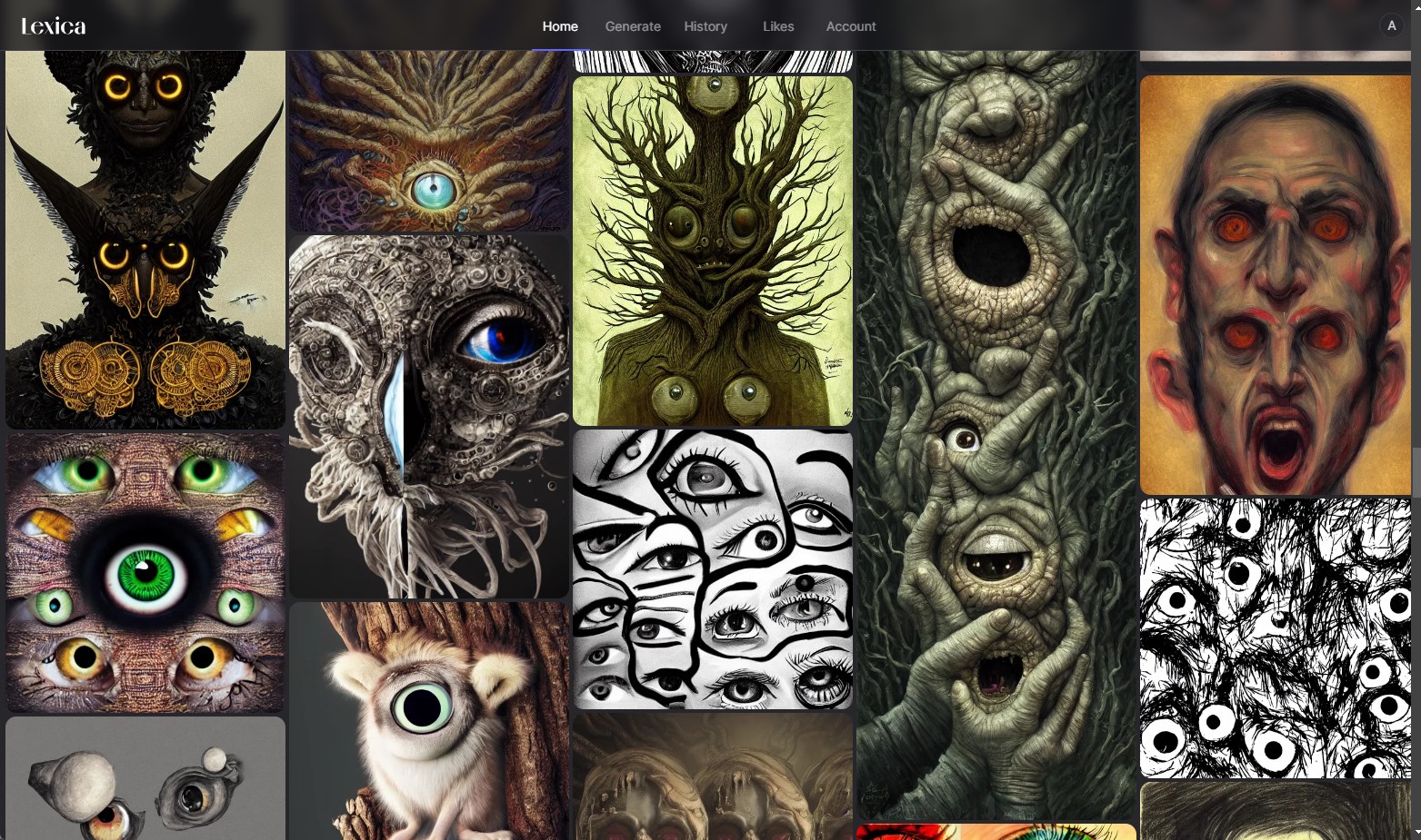
The current solution is to either go through a prompt guide and learn the styles people found successful in the past, or search a gallery like Lexica that contains millions of examples and their respective prompts. I go for the latter as learning arcane keywords that would work on specific versions of specific models is not a winning strategy for the long term.
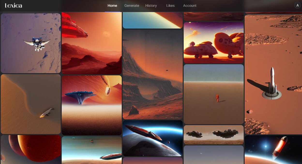
From here, I find an image that I like, and edit it with my subject keeping the style portion of the prompt, so finally it looks like:
fighter jets flying over a red planet in space flaming jets behind them, stars on a black sky, lava, ussr, soviet, as a realistic scifi spaceship!!!, floating in space, wide angle shot art, vintage retro scifi, realistic space, digital art, trending on artstation, symmetry!!! dramatic lighting.
The results of Midjourney have always stood out as especially beautiful. I tried it with the original prompt containing only the subject. The results were amazing.
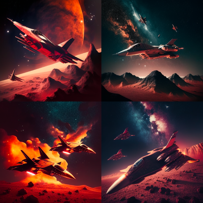
While these look incredible, they don’t capture the essence of the original image as well as the Stable Diffusion one does. But this convinced me to try Midjourney first for the remainder of the story. I had about eight images to generate and only a limited time to get an okay result for each.
Original Image:
Final Image:
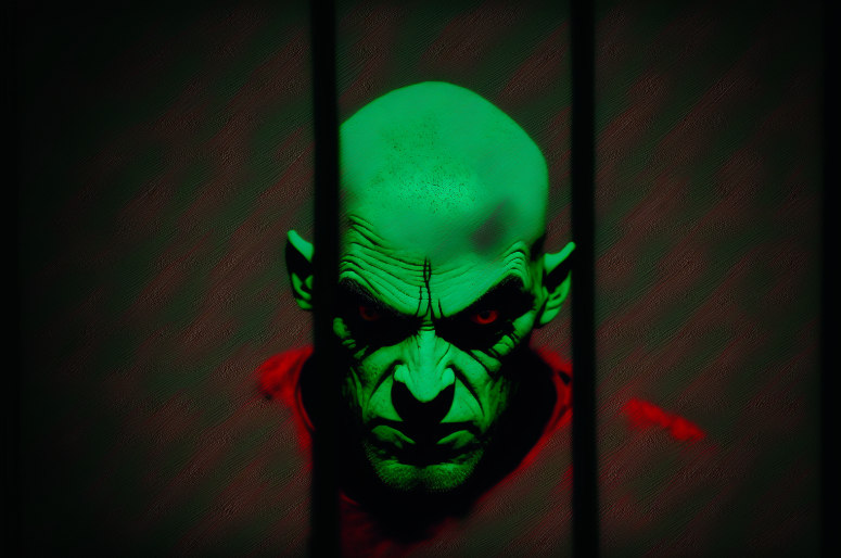
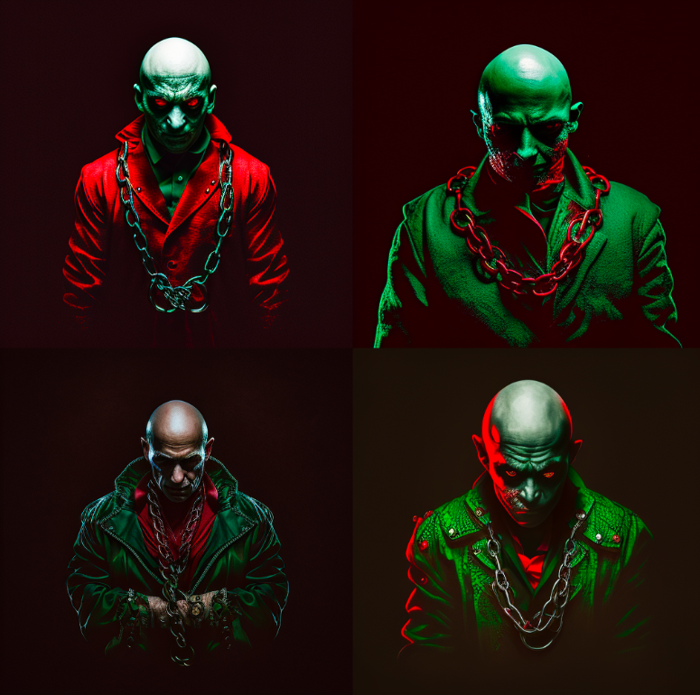
While Midjourney could approximate the appearance of Dr. Venom, it was difficult to get the pose and restraint. My attempts at that looked like this:
That’s why I tweaked the image to show him behind bars instead.
Original Image:
Final Image:
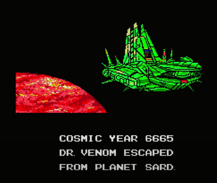
To instruct the model to generate a wide image, the –ar 3:2 command specifies the desired aspect ratio.
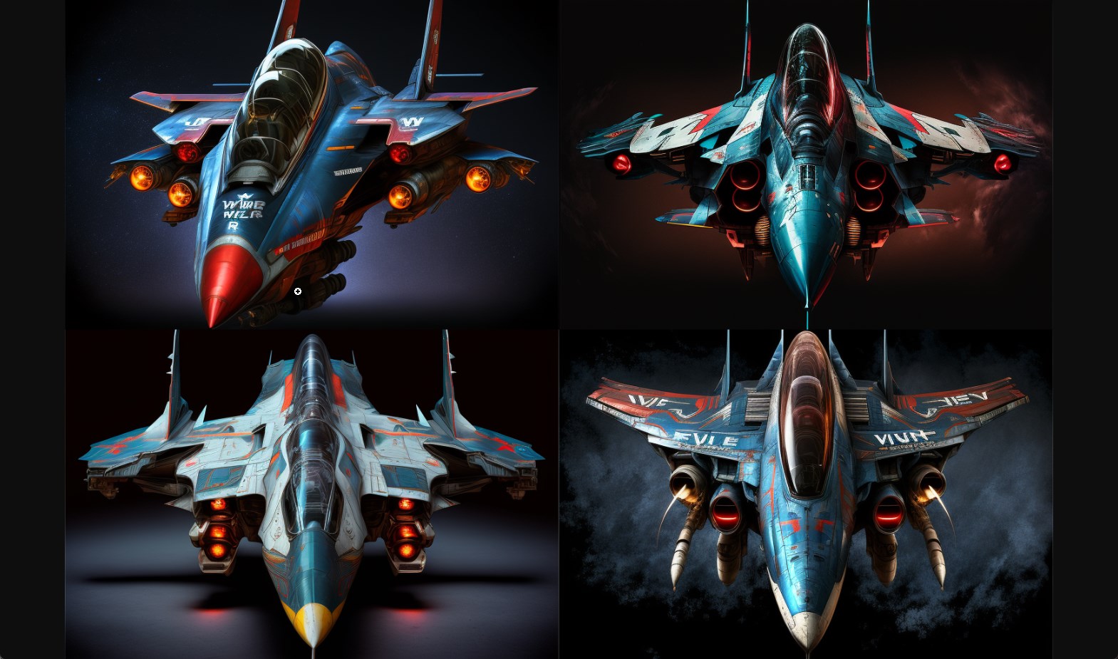
Original Image:
Final Image:
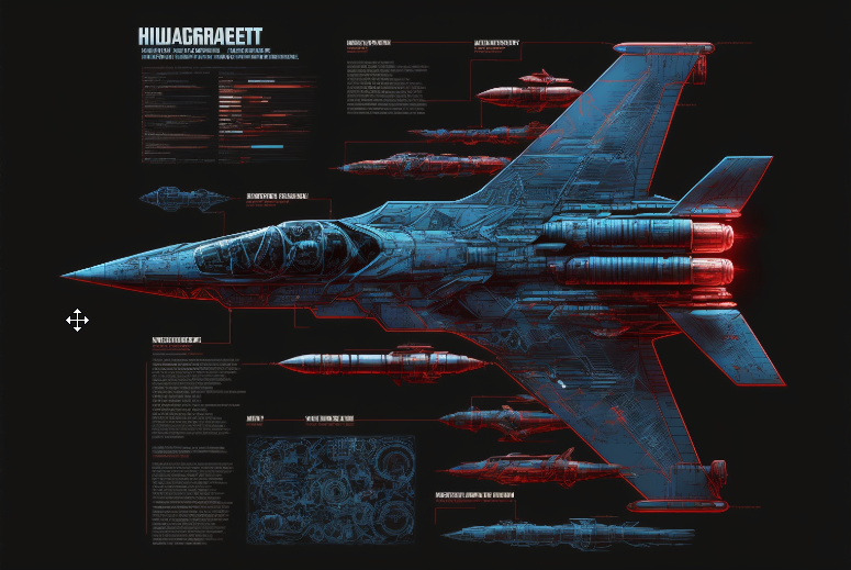
Midjourney really captures the cool factor in a lot of fighter jet schematics. The text will not make sense, but that can work in your favor if you’re going for something alien.
In this workflow, it’ll be difficult to reproduce the same plane in future panels. Recent, more advanced methods like textual inversion or photobooth could aid in this, but at this time they are more difficult to use than text-to-image services.
Original Image:
Final Image:
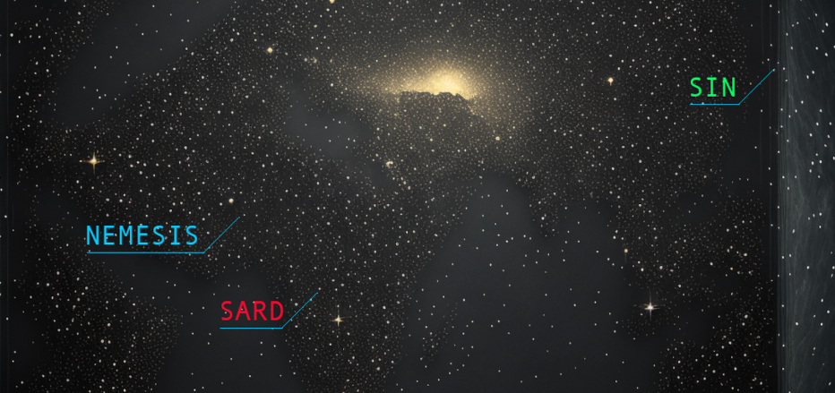
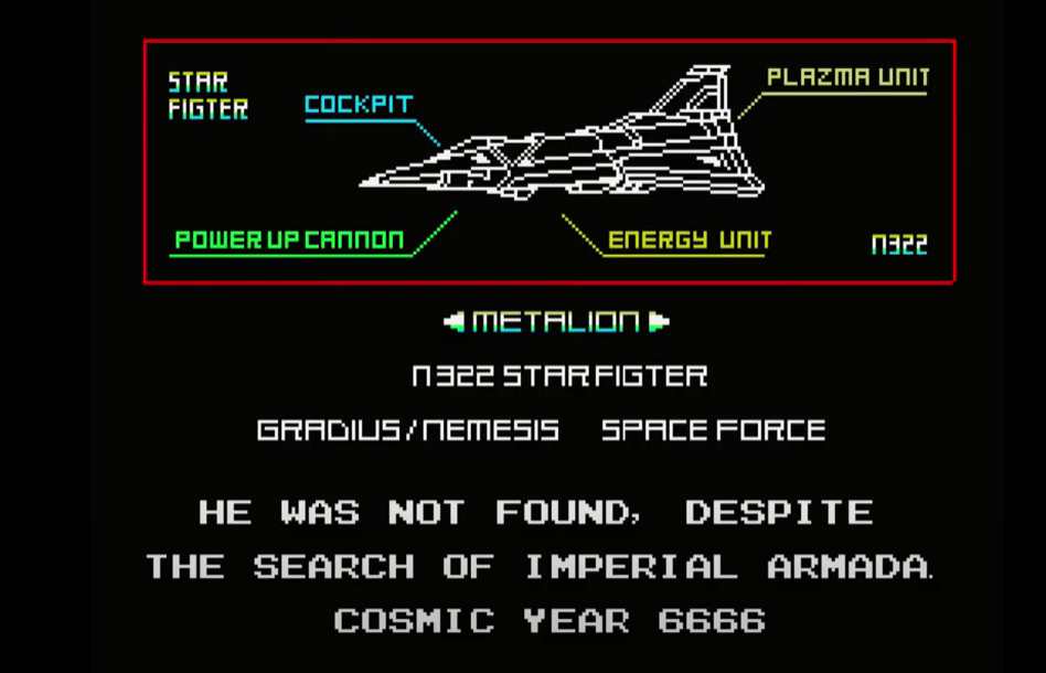
This image shows a limitation in what is possible with the current batch of AI image tools:
1- Reproducing text correctly in images is still not yet widely available (although technically possible as demonstrated in Google’s Imagen)
2- Text-to-image is not the best paradigm if you need a specific placement or manipulation of elements
So to get this final image, I had to import the stars image into photoshop and add the text and lines there.
Original Image:
I failed at reproducing the most iconic portion of this image, the three eyes. The models wouldn’t generate the look using any of the prompts I’ve tried.
I then proceeded to try in-painting in Dream Studio.
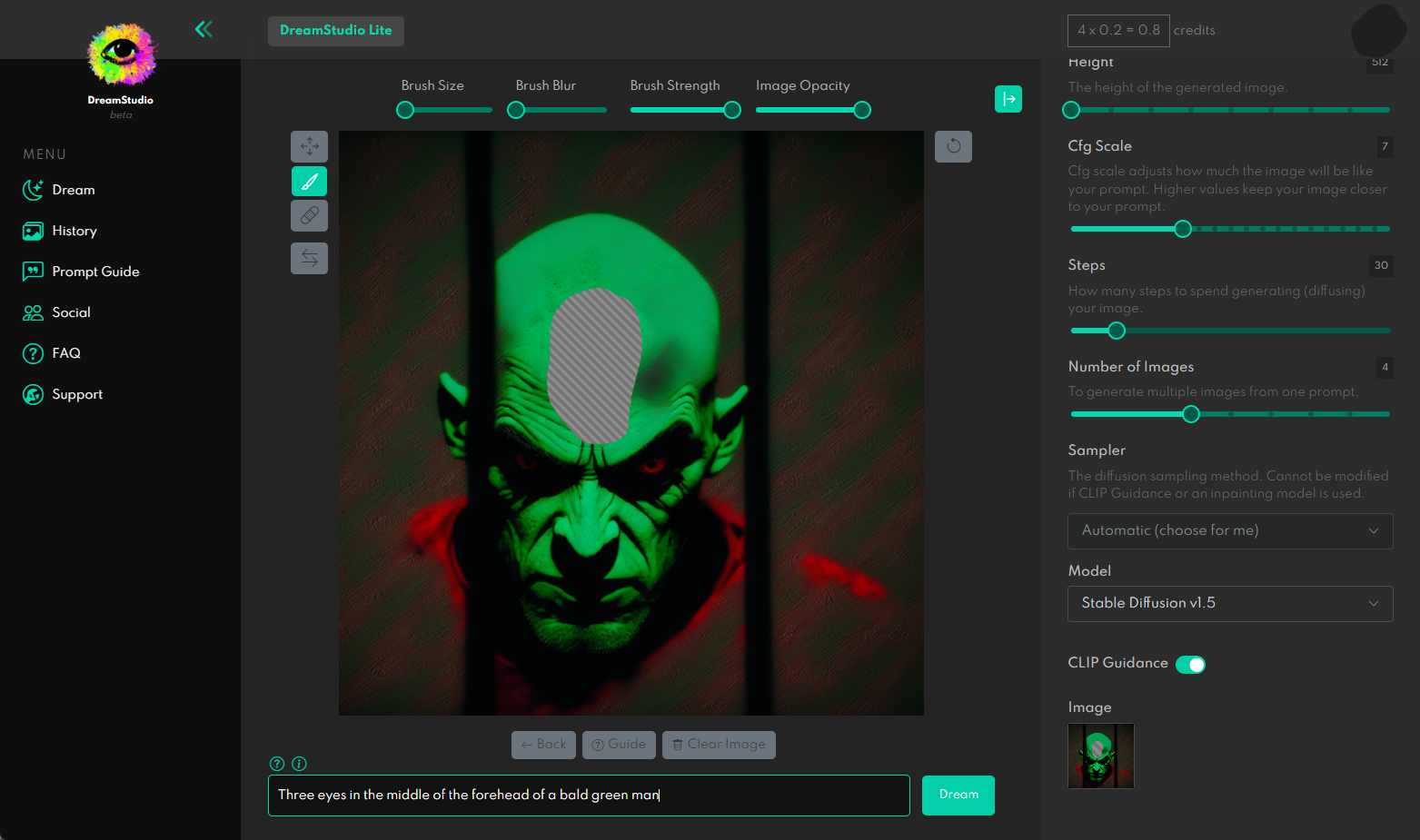
In-painting instructs the model to only generate an image for a portion of the image, in this case, it’s the portion I deleted with the brush inside of Dream Studio above.
I couldn’t get to a good result in time. Although looking at the gallery, the models are quite capable of generating horrific imagery involving eyes.
Original Image:
Candidate generations:
Original Image:
Candidate generations:
This image provided a good opportunity to try out DALL-E’s outpainting tool to expand the canvas and fill-in the surrounding space with content.
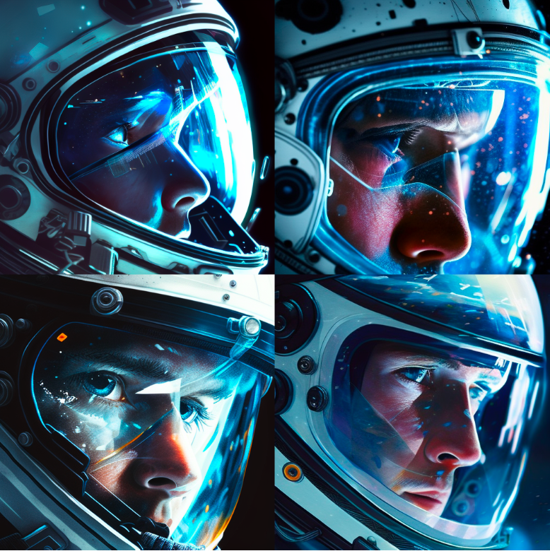
Say we decided to go with this image for the ship’s captain

We can upload it to DALL-E’s outpainting editor and over a number of generations continue to expand the imagery around the image (taking into consideration a part of the image so we keep some continuity).
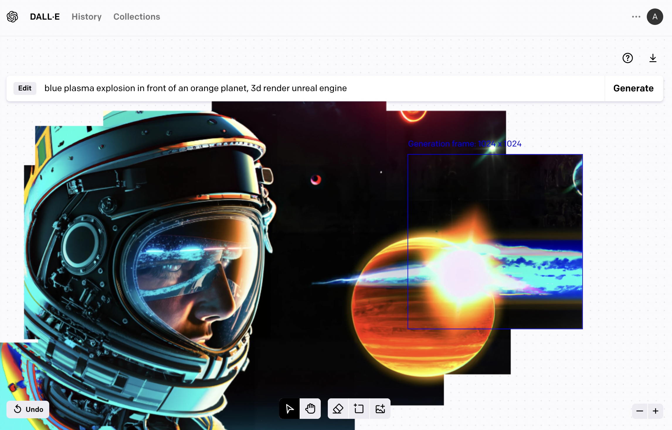
The outpainting workflow is different from the text2image in that the prompt has to be changed to describe the portion you’re crafting at each portion of the image.
It’s been a few months since the vast majority of people started having broad access to AI image generation tools. The major milestone here is the open source release of Stable Diffusion (although some people had access to DALL-E before, and models like OpenAI GLIDE were publicly available but slower and less capable). During this time, I’ve gotten to use three of these image generation services.
This is what I have been using the most over the last few months.

That said, do not discount DALL-E just yet, however. OpenAI are quite the pioneers and I’d expect the next versions of the model to dramatically improve generation quality.
This is a good place to end this post although there are a bunch of other topics I had wanted to address. Let me know what you think on @JayAlammar or @JayAlammar@sigmoid.social.
]]>(V2 Nov 2022: Updated images for more precise description of forward diffusion. A few more images in this version)
AI image generation is the most recent AI capability blowing people’s minds (mine included). The ability to create striking visuals from text descriptions has a magical quality to it and points clearly to a shift in how humans create art. The release of Stable Diffusion is a clear milestone in this development because it made a high-performance model available to the masses (performance in terms of image quality, as well as speed and relatively low resource/memory requirements).
After experimenting with AI image generation, you may start to wonder how it works.
This is a gentle introduction to how Stable Diffusion works.
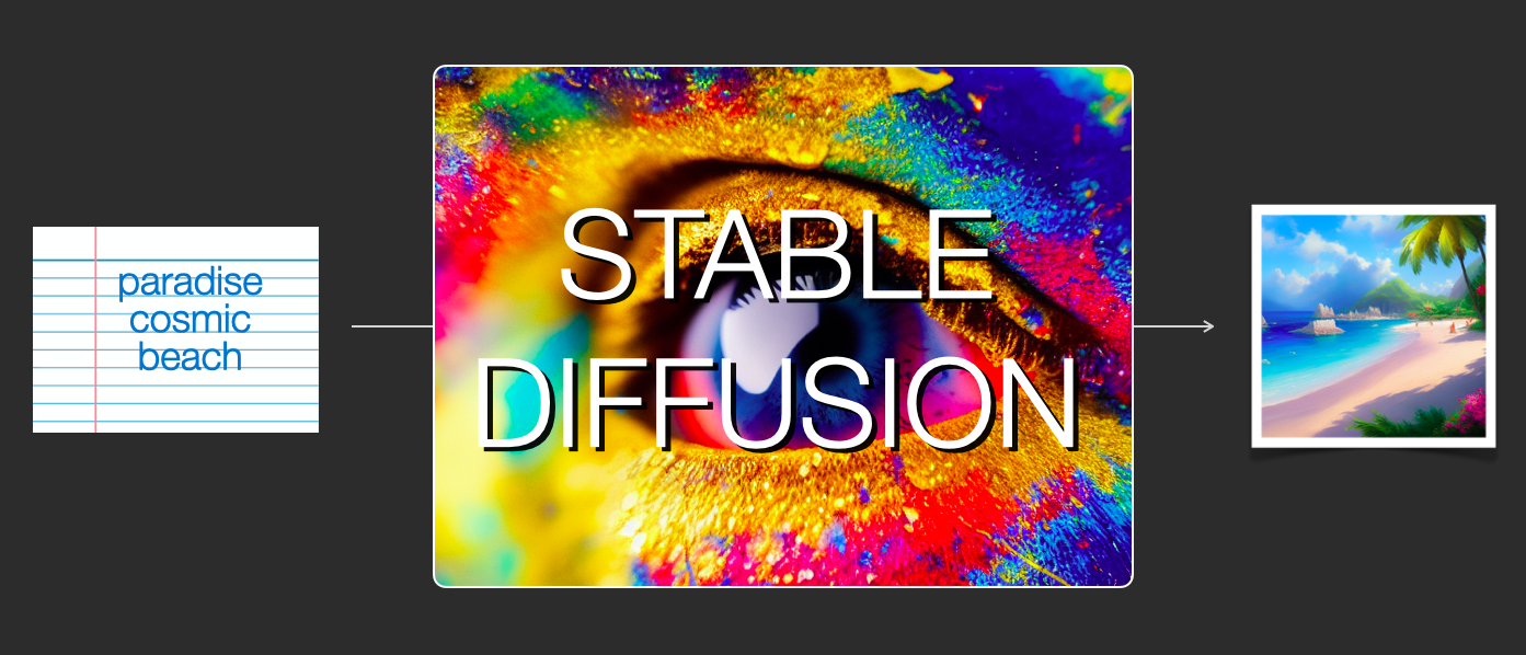
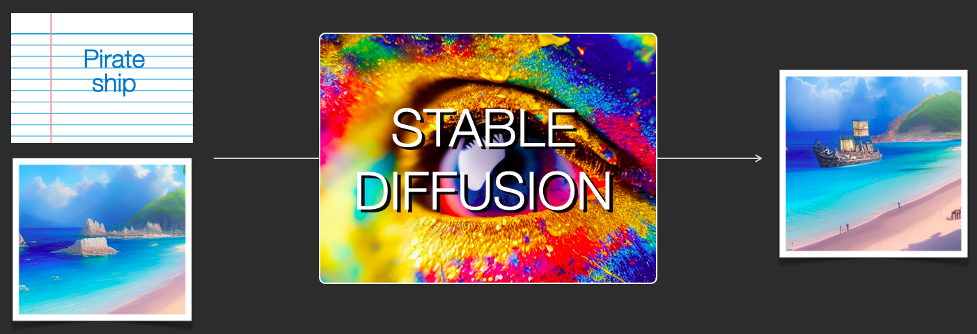
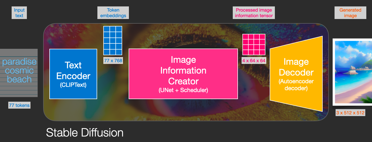
Stable Diffusion is versatile in that it can be used in a number of different ways. Let’s focus at first on image generation from text only (text2img). The image above shows an example text input and the resulting generated image (The actual complete prompt is here). Aside from text to image, another main way of using it is by making it alter images (so inputs are text + image).
Let’s start to look under the hood because that helps explain the components, how they interact, and what the image generation options/parameters mean.
Stable Diffusion is a system made up of several components and models. It is not one monolithic model.
As we look under the hood, the first observation we can make is that there’s a text-understanding component that translates the text information into a numeric representation that captures the ideas in the text.
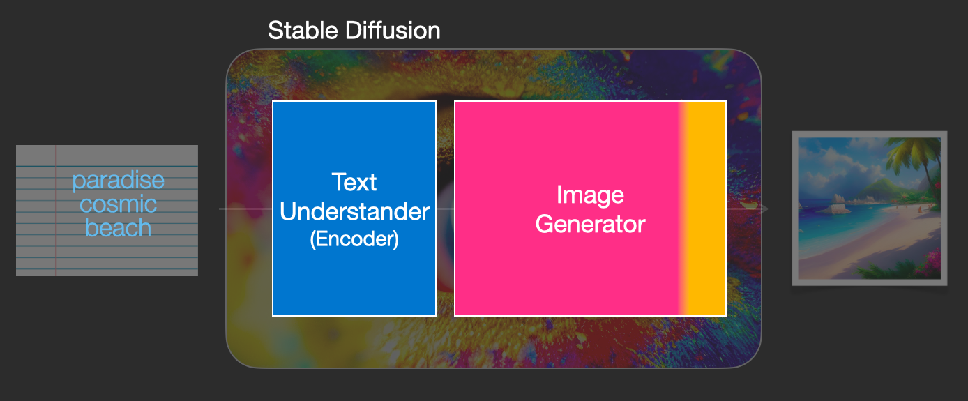
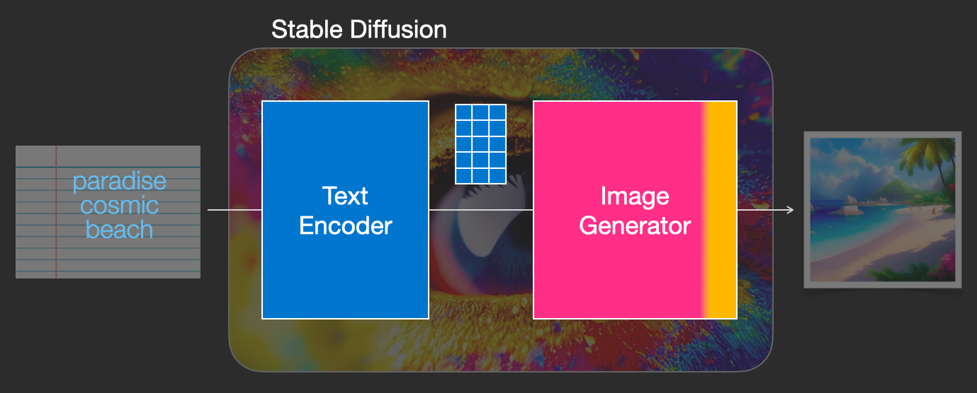
We’re starting with a high-level view and we’ll get into more machine learning details later in this article. However, we can say that this text encoder is a special Transformer language model (technically: the text encoder of a CLIP model). It takes the input text and outputs a list of numbers representing each word/token in the text (a vector per token).
That information is then presented to the Image Generator, which is composed of a couple of components itself.
The image generator goes through two stages:
1- Image information creator
This component is the secret sauce of Stable Diffusion. It’s where a lot of the performance gain over previous models is achieved.
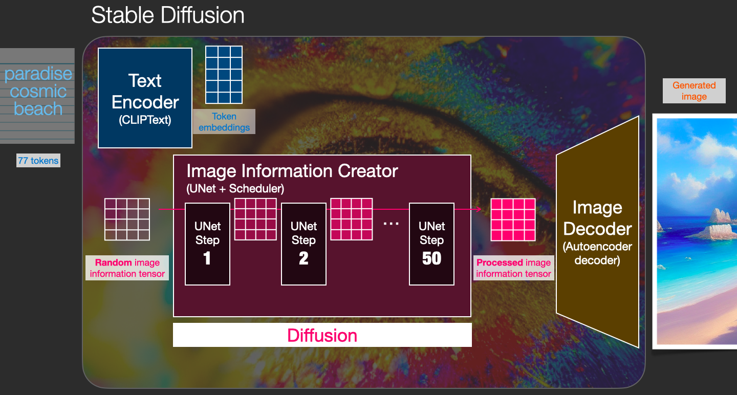
This component runs for multiple steps to generate image information. This is the steps parameter in Stable Diffusion interfaces and libraries which often defaults to 50 or 100.
The image information creator works completely in the image information space (or latent space). We’ll talk more about what that means later in the post. This property makes it faster than previous diffusion models that worked in pixel space. In technical terms, this component is made up of a UNet neural network and a scheduling algorithm.
The word “diffusion” describes what happens in this component. It is the step by step processing of information that leads to a high-quality image being generated in the end (by the next component, the image decoder).
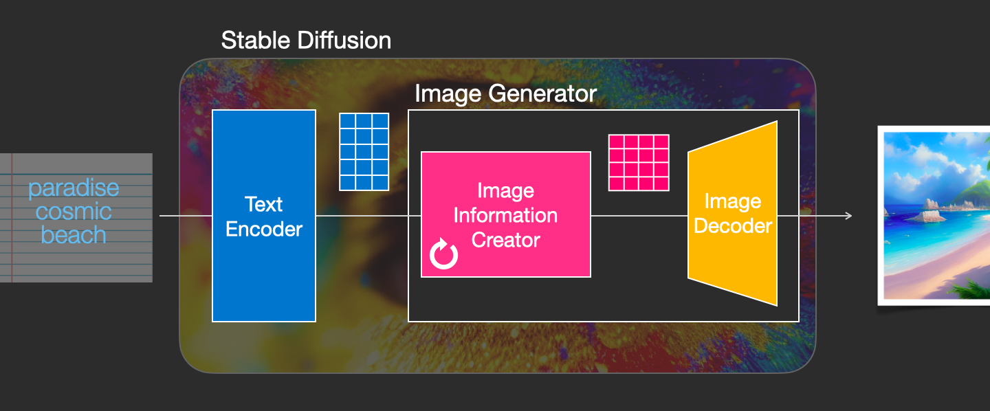
2- Image Decoder
The image decoder paints a picture from the information it got from the information creator. It runs only once at the end of the process to produce the final pixel image.
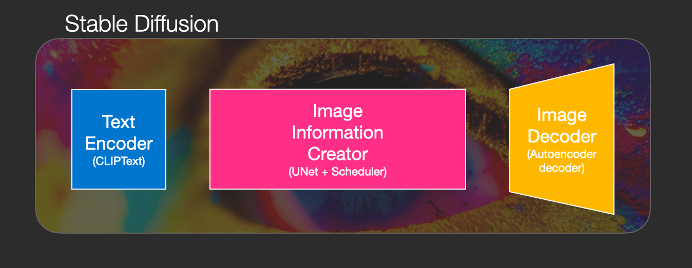
With this we come to see the three main components (each with its own neural network) that make up Stable Diffusion:
ClipText for text encoding.
Input: text.
Output: 77 token embeddings vectors, each in 768 dimensions.
UNet + Scheduler to gradually process/diffuse information in the information (latent) space.
Input: text embeddings and a starting multi-dimensional array (structured lists of numbers, also called a tensor) made up of noise.
Output: A processed information array
Autoencoder Decoder that paints the final image using the processed information array.
Input: The processed information array (dimensions: (4,64,64))
Output: The resulting image (dimensions: (3, 512, 512) which are (red/green/blue, width, height))
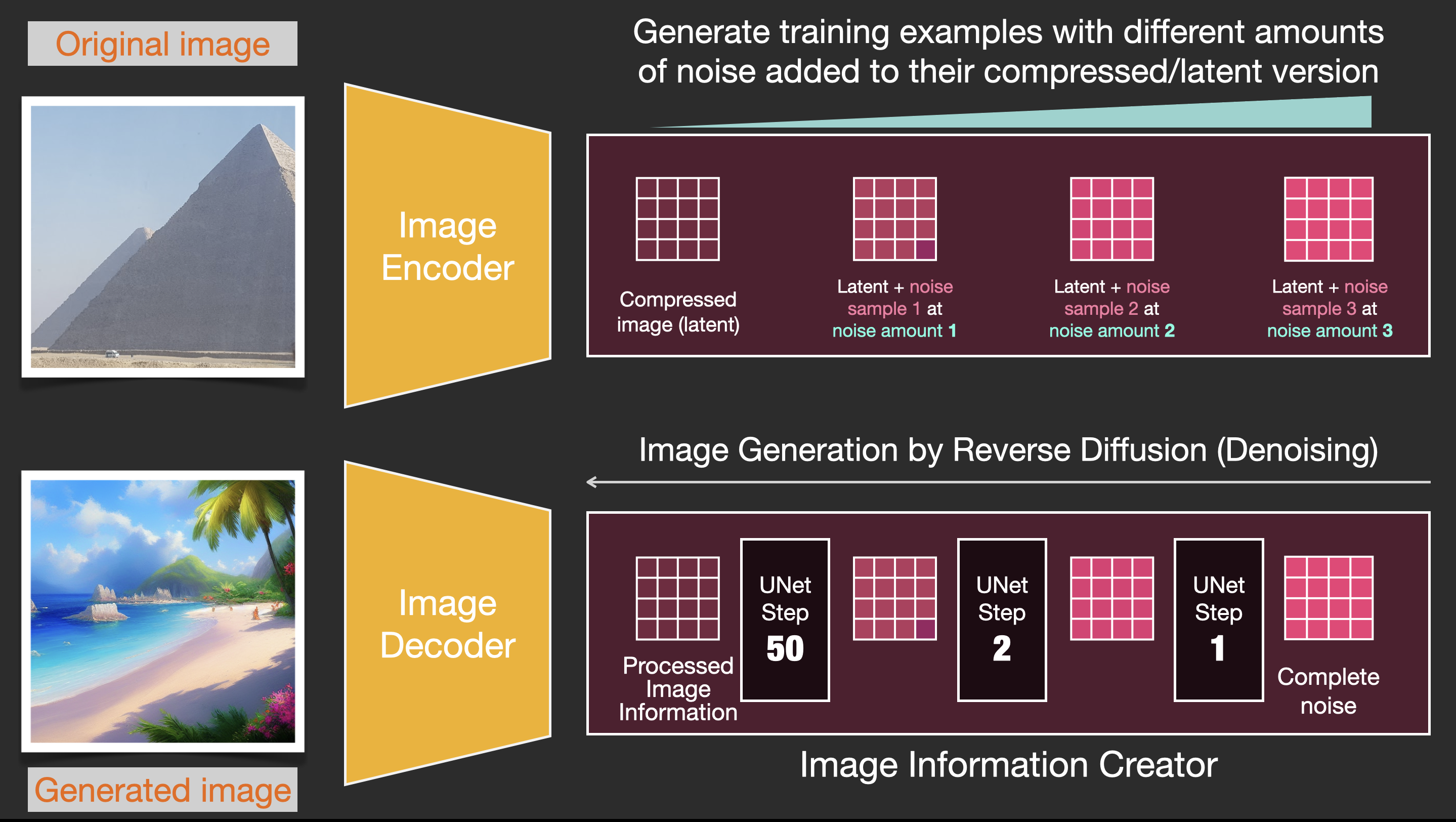
Diffusion is the process that takes place inside the pink “image information creator” component. Having the token embeddings that represent the input text, and a random starting image information array (these are also called latents), the process produces an information array that the image decoder uses to paint the final image.
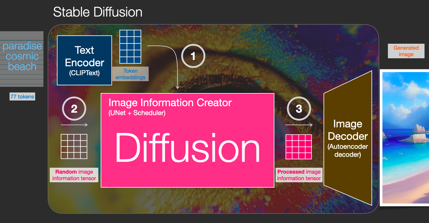
This process happens in a step-by-step fashion. Each step adds more relevant information. To get an intuition of the process, we can inspect the random latents array, and see that it translates to visual noise. Visual inspection in this case is passing it through the image decoder.
Diffusion happens in multiple steps, each step operates on an input latents array, and produces another latents array that better resembles the input text and all the visual information the model picked up from all images the model was trained on.
We can visualize a set of these latents to see what information gets added at each step.
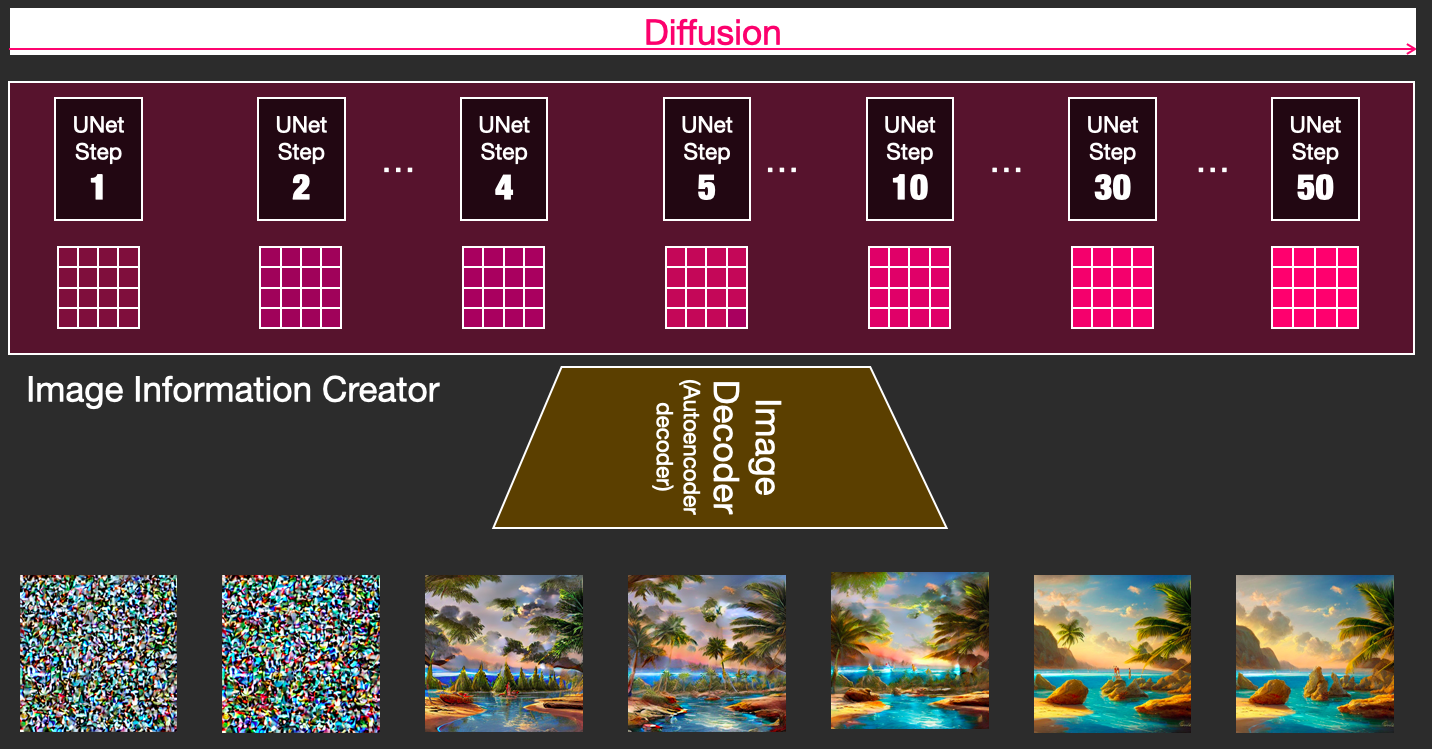
The process is quite breathtaking to look at.
Something especially fascinating happens between steps 2 and 4 in this case. It’s as if the outline emerges from the noise.
The central idea of generating images with diffusion models relies on the fact that we have powerful computer vision models. Given a large enough dataset, these models can learn complex operations. Diffusion models approach image generation by framing the problem as following:
Say we have an image, we generate some noise, and add it to the image.
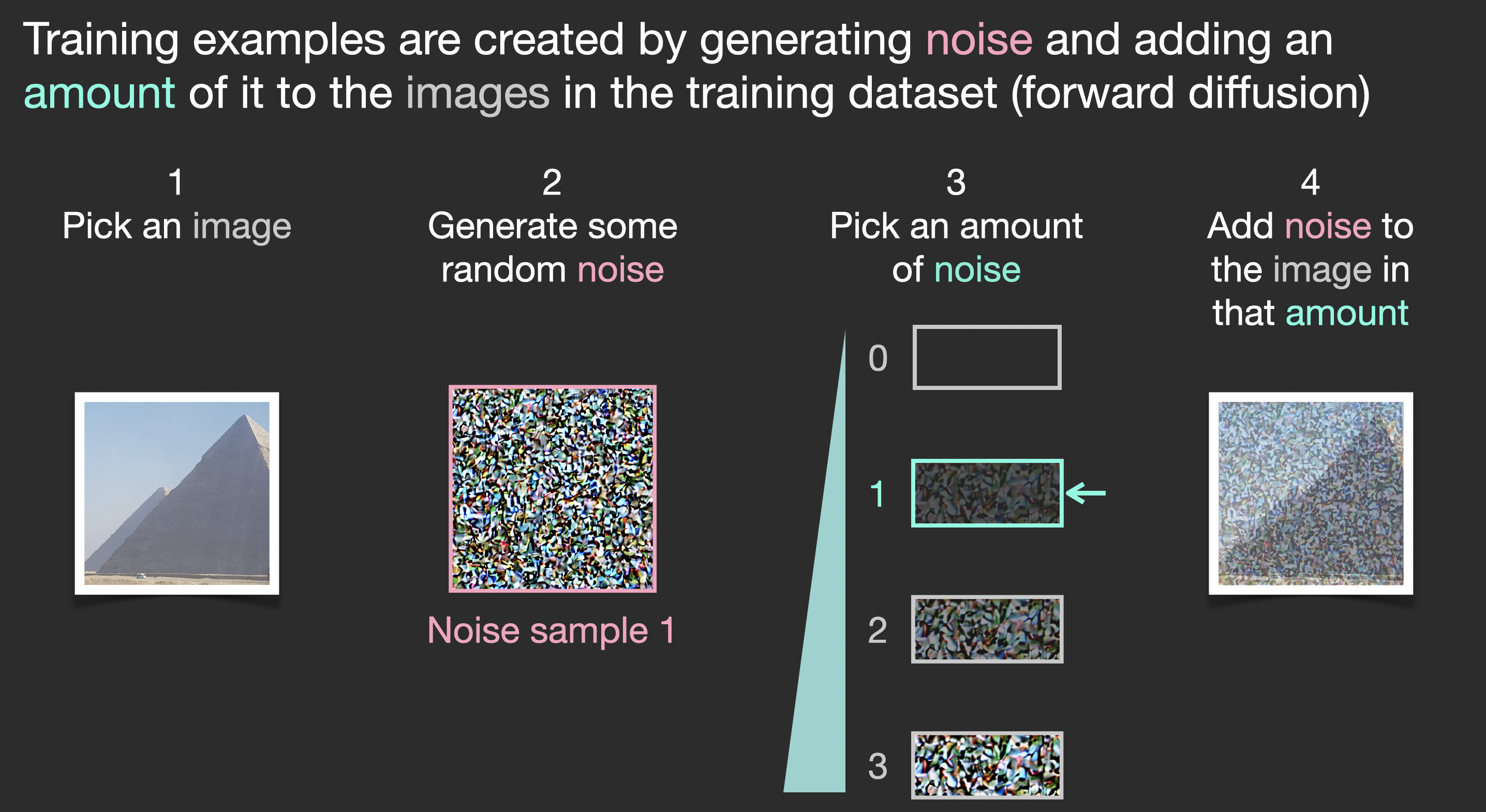
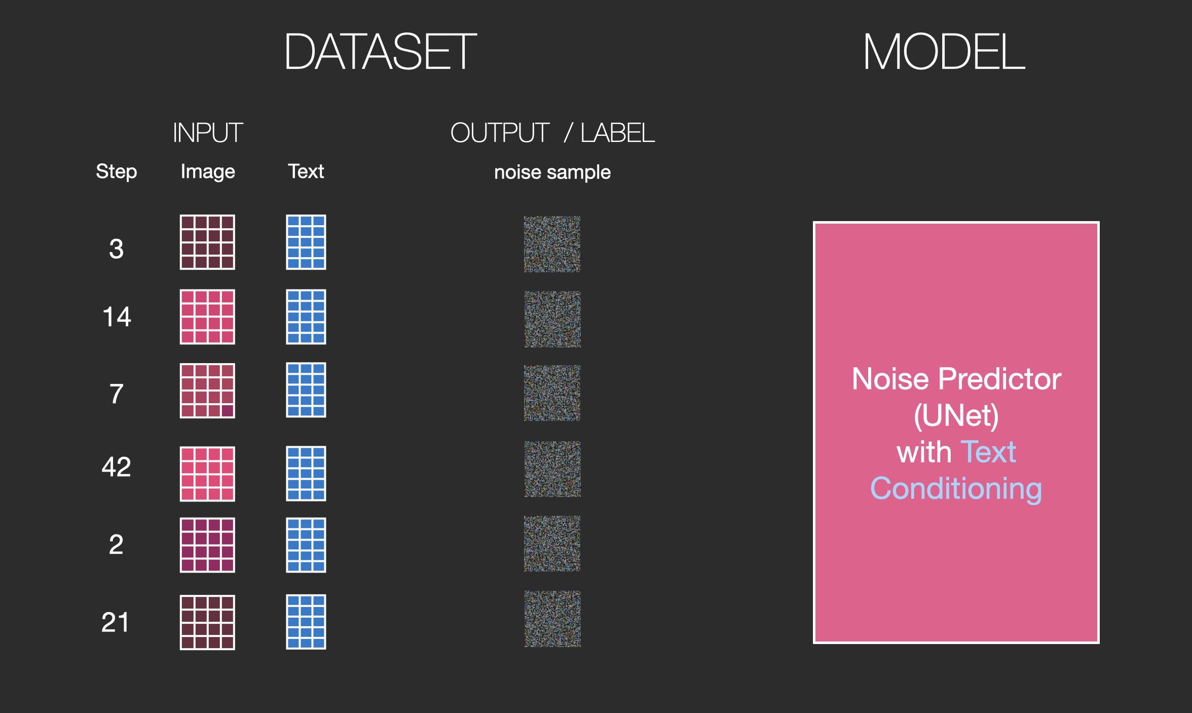
This can now be considered a training example. We can use this same formula to create lots of training examples to train the central component of our image generation model.
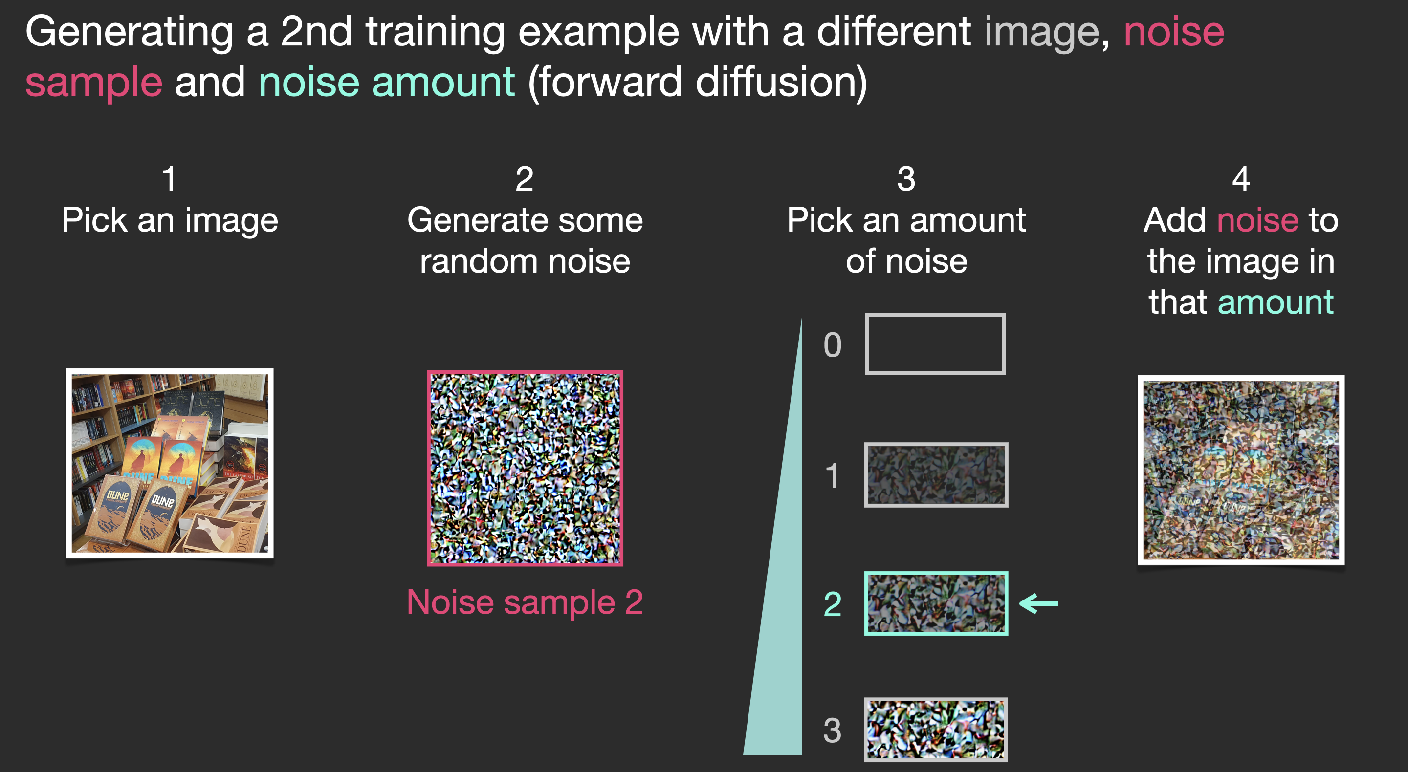
While this example shows a few noise amount values from image (amount 0, no noise) to total noise (amount 4, total noise), we can easily control how much noise to add to the image, and so we can spread it over tens of steps, creating tens of training examples per image for all the images in a training dataset.
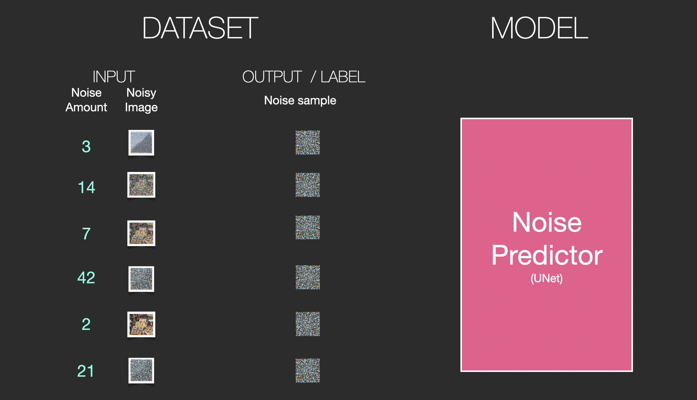
With this dataset, we can train the noise predictor and end up with a great noise predictor that actually creates images when run in a certain configuration. A training step should look familiar if you’ve had ML exposure:
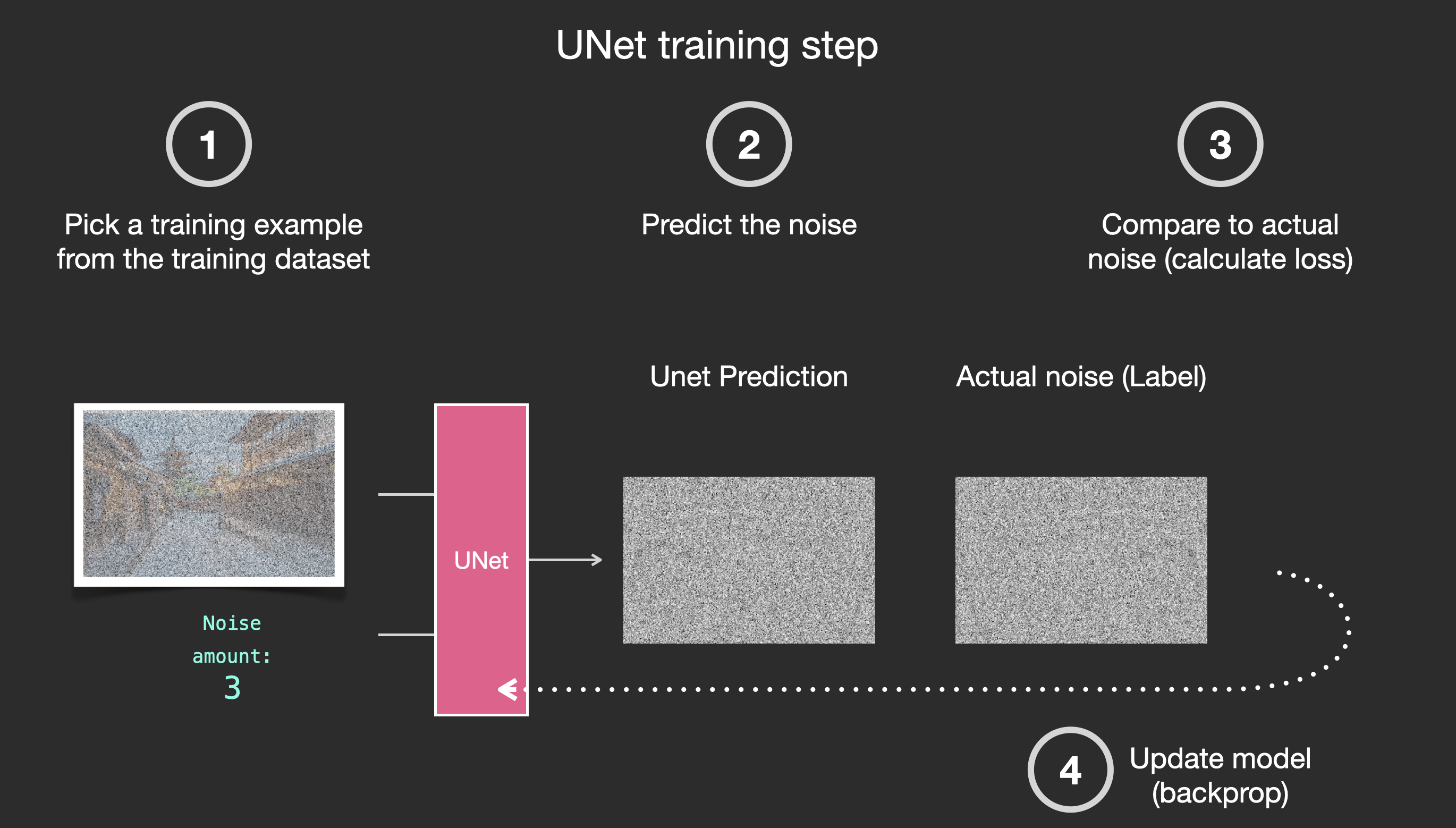
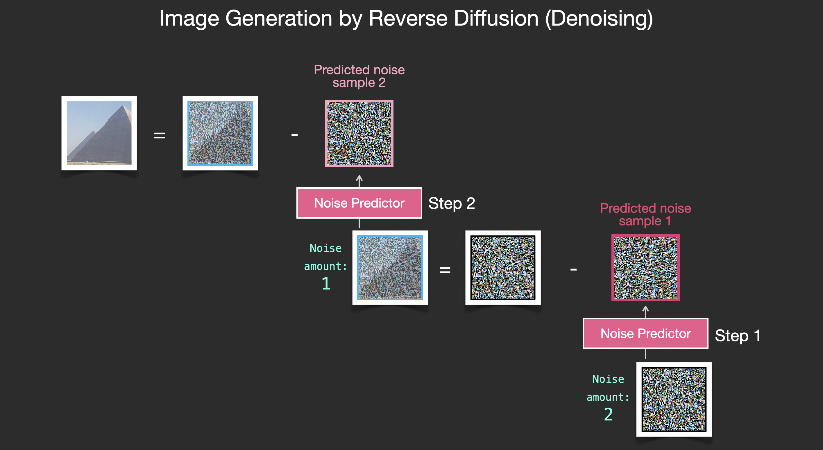
Let’s now see how this can generate images.
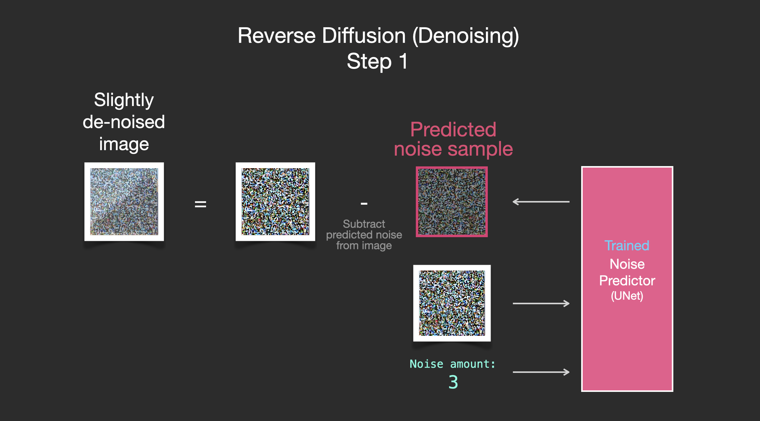
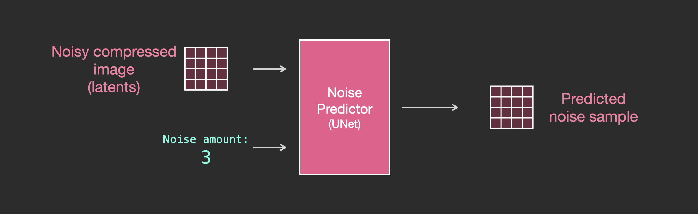
The trained noise predictor can take a noisy image, and the number of the denoising step, and is able to predict a slice of noise.
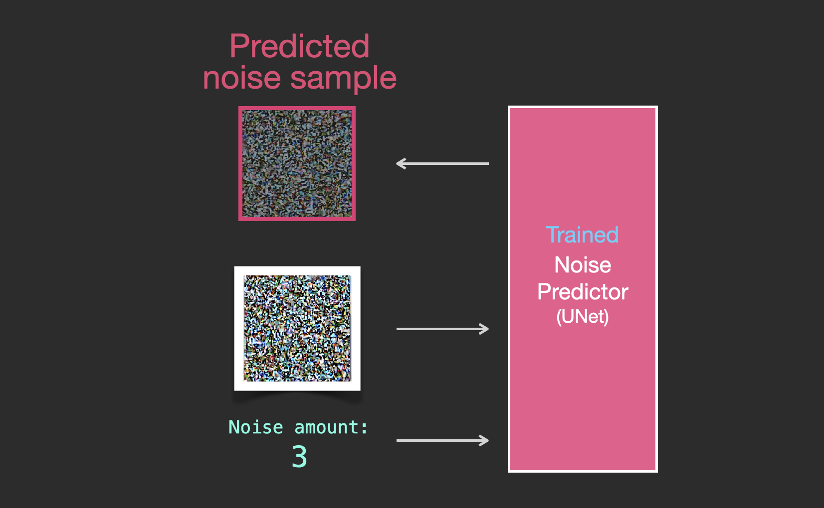
The sampled noise is predicted so that if we subtract it from the image, we get an image that’s closer to the images the model was trained on (not the exact images themselves, but the distribution - the world of pixel arrangements where the sky is usually blue and above the ground, people have two eyes, cats look a certain way – pointy ears and clearly unimpressed).
If the training dataset was of aesthetically pleasing images (e.g., LAION Aesthetics, which Stable Diffusion was trained on), then the resulting image would tend to be aesthetically pleasing. If the we train it on images of logos, we end up with a logo-generating model.
This concludes the description of image generation by diffusion models mostly as described in Denoising Diffusion Probabilistic Models. Now that you have this intuition of diffusion, you know the main components of not only Stable Diffusion, but also Dall-E 2 and Google’s Imagen.
Note that the diffusion process we described so far generates images without using any text data. So if we deploy this model, it would generate great looking images, but we’d have no way of controlling if it’s an image of a pyramid or a cat or anything else. In the next sections we’ll describe how text is incorporated in the process in order to control what type of image the model generates.
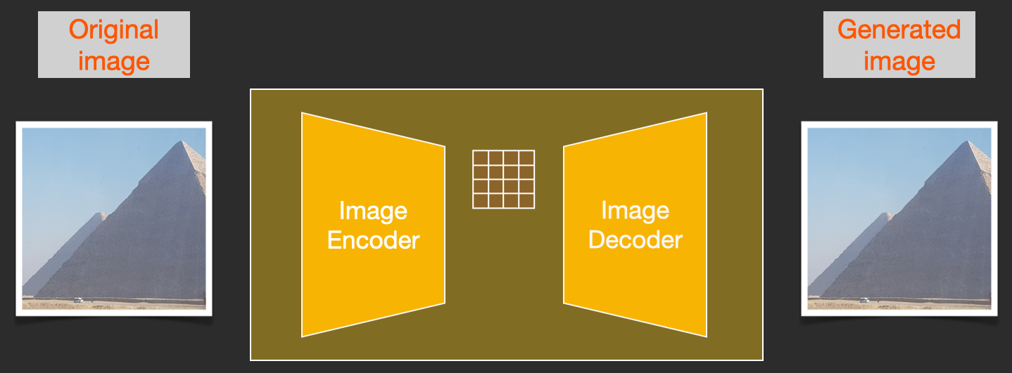
To speed up the image generation process, the Stable Diffusion paper runs the diffusion process not on the pixel images themselves, but on a compressed version of the image. The paper calls this “Departure to Latent Space”.
This compression (and later decompression/painting) is done via an autoencoder. The autoencoder compresses the image into the latent space using its encoder, then reconstructs it using only the compressed information using the decoder.
Now the forward diffusion process is done on the compressed latents. The slices of noise are of noise applied to those latents, not to the pixel image. And so the noise predictor is actually trained to predict noise in the compressed representation (the latent space).

The forward process (using the autoencoder’s encoder) is how we generate the data to train the noise predictor. Once it’s trained, we can generate images by running the reverse process (using the autoencoder’s decoder).
These two flows are what’s shown in Figure 3 of the LDM/Stable Diffusion paper:
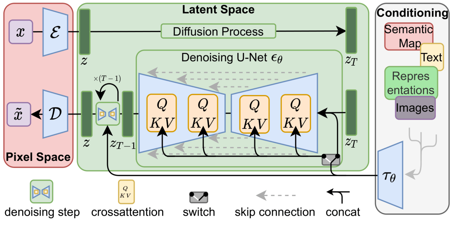
This figure additionally shows the “conditioning” components, which in this case is the text prompts describing what image the model should generate. So let’s dig into the text components.
A Transformer language model is used as the language understanding component that takes the text prompt and produces token embeddings. The released Stable Diffusion model uses ClipText (A GPT-based model), while the paper used BERT.
The choice of language model is shown by the Imagen paper to be an important one. Swapping in larger language models had more of an effect on generated image quality than larger image generation components.
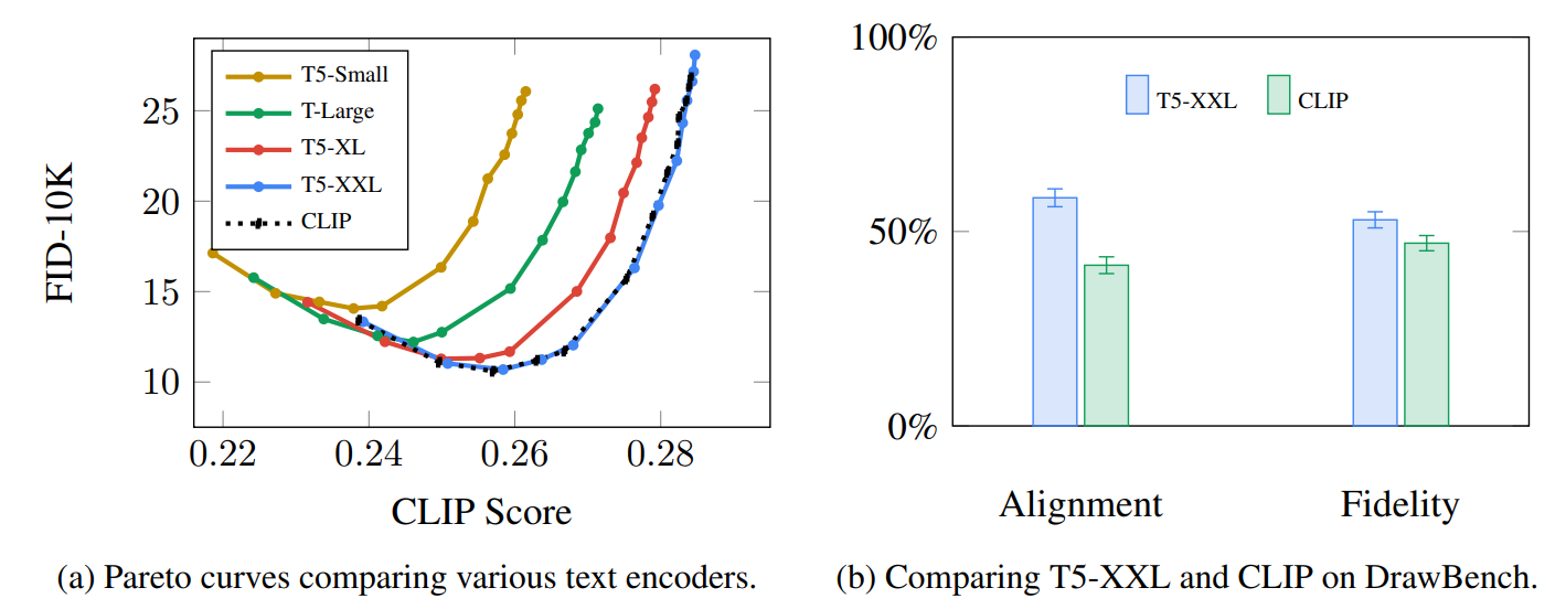
The early Stable Diffusion models just plugged in the pre-trained ClipText model released by OpenAI. It’s possible that future models may switch to the newly released and much larger OpenCLIP variants of CLIP (Nov2022 update: True enough, Stable Diffusion V2 uses OpenClip). This new batch includes text models of sizes up to 354M parameters, as opposed to the 63M parameters in ClipText.
CLIP is trained on a dataset of images and their captions. Think of a dataset looking like this, only with 400 million images and their captions:
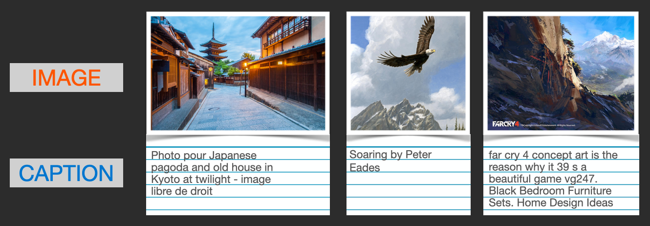
In actuality, CLIP was trained on images crawled from the web along with their “alt” tags.
CLIP is a combination of an image encoder and a text encoder. Its training process can be simplified to thinking of taking an image and its caption. We encode them both with the image and text encoders respectively.
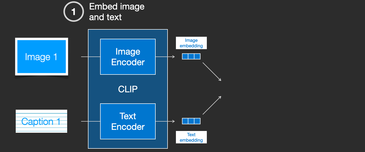
We then compare the resulting embeddings using cosine similarity. When we begin the training process, the similarity will be low, even if the text describes the image correctly.
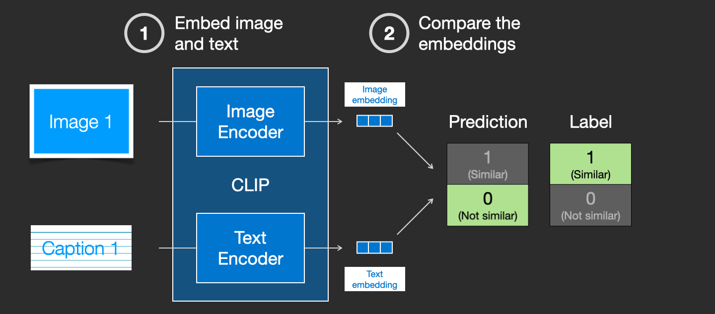
We update the two models so that the next time we embed them, the resulting embeddings are similar.
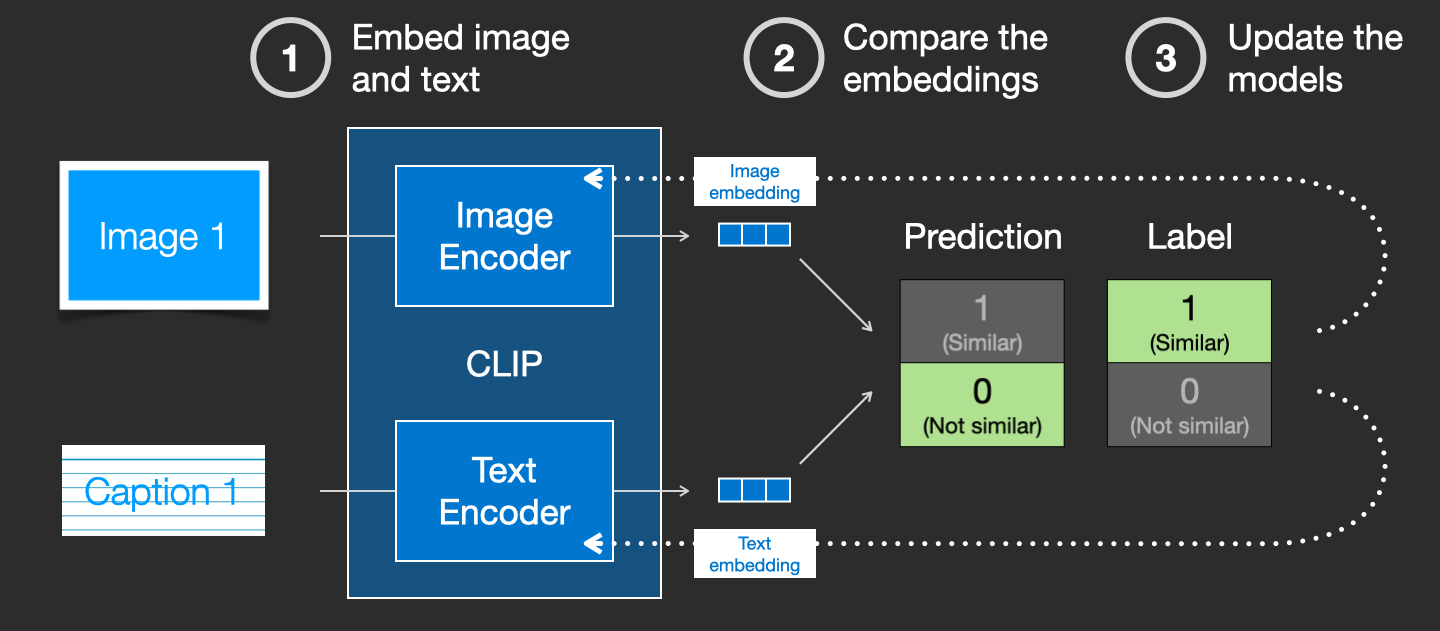
By repeating this across the dataset and with large batch sizes, we end up with the encoders being able to produce embeddings where an image of a dog and the sentence “a picture of a dog” are similar. Just like in word2vec, the training process also needs to include negative examples of images and captions that don’t match, and the model needs to assign them low similarity scores.
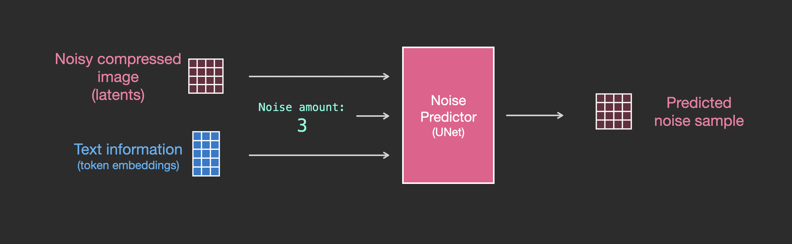
To make text a part of the image generation process, we have to adjust our noise predictor to use the text as an input.
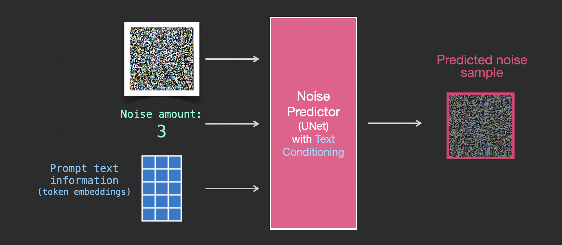
Our dataset now includes the encoded text. Since we’re operating in the latent space, both the input images and predicted noise are in the latent space.
To get a better sense of how the text tokens are used in the Unet, let’s look deeper inside the Unet.
Let’s first look at a diffusion Unet that does not use text. Its inputs and outputs would look like this:
Inside, we see that:
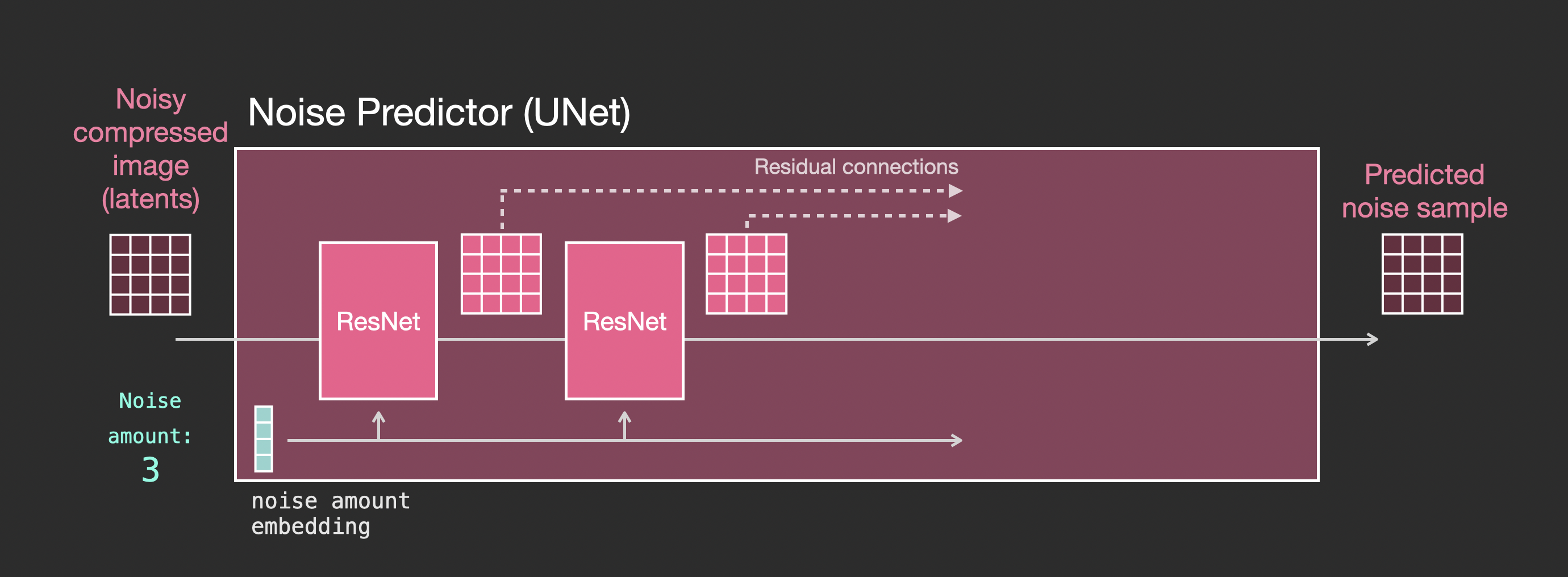
Let’s now look how to alter this system to include attention to the text.
The main change to the system we need to add support for text inputs (technical term: text conditioning) is to add an attention layer between the ResNet blocks.
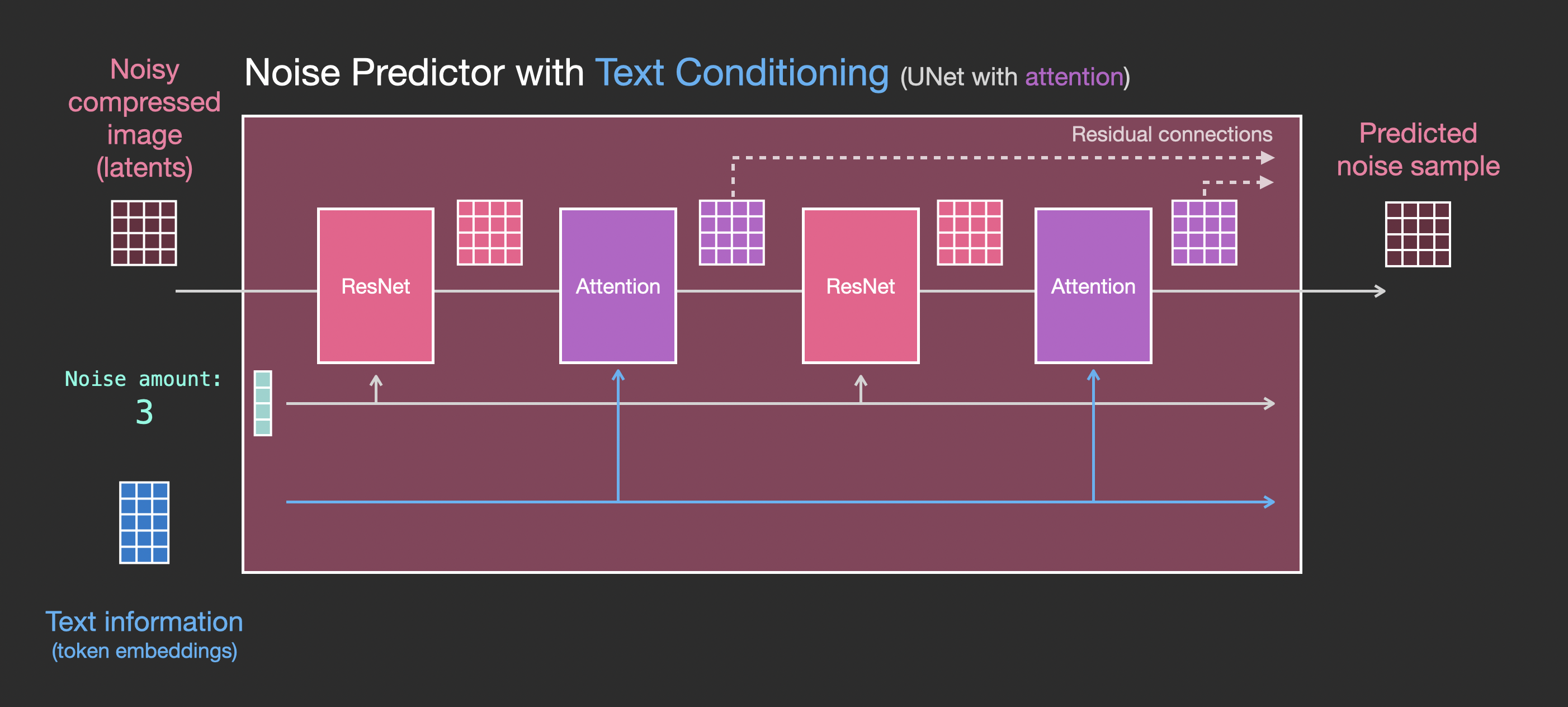
Note that the ResNet block doesn’t directly look at the text. But the attention layers merge those text representations in the latents. And now the next ResNet can utilize that incorporated text information in its processing.
I hope this gives you a good first intuition about how Stable Diffusion works. Lots of other concepts are involved, but I believe they’re easier to understand once you’re familiar with the building blocks above. The resources below are great next steps that I found useful. Please reach out to me on Twitter for any corrections or feedback.
Thanks to Robin Rombach, Jeremy Howard, Hamel Husain, Dennis Soemers, Yan Sidyakin, Freddie Vargus, Anna Golubeva, and the Cohere For AI community for feedback on earlier versions of this article.
Please help me make this article better. Possible ways:
If you’re interested in discussing the overlap of image generation models with language models, feel free to post in the #images-and-words channel in the Cohere community on Discord. There, we discuss areas of overlap, including:
If you found this work helpful for your research, please cite it as following:
@misc{alammar2022diffusion,
  title={The Illustrated Stable Diffusion},
  author={Alammar, J},
  year={2022},
  url={https://jalammar.github.io/illustrated-stable-diffusion/}
}
I love that I get to share some of the intuitions developers need to start problem-solving with these models. Even though I’ve been working very closely on pretrained Transformers for the past several years (for this blog and in developing Ecco), I’m enjoying the convenience of problem-solving with managed language models as it frees up the restrictions of model loading/deployment and memory/GPU management.
These are some of the articles I wrote and collaborated on with colleagues over the last few months:

This is a high-level intro to large language models to people who are new to them. It establishes the difference between generative (GPT-like) and representation (BERT-like) models and examples use cases for them.
This is one of the first articles I got to write. It's extracted from a much larger document that I wrote to explore some of the visual language to use in explaining the application of these models.

Massive GPT models open the door for a new way of programming. If you structure the input text in the right way, you can useful (and often fascinating) results for a lot of taasks (e.g. text classification, copy writing, summarization...etc).
This article visually demonstrates four principals to create prompts effectively.

This is a walkthrough of creating a simple summarization system. It links to a jupyter notebook which includes the code to start experimenting with text generation and summarization.
The end of this notebook shows an important idea I want to spend more time on in the future. That of how to rank/filter/select the best from amongst multiple generations.

Semantic search has to be one of the most exciting applications of sentence embedding models. This tutorials implements a "similar questions" functionality using sentence embeddings and a a vector search library.
The vector search library used here is Annoy from Spotify. There are a bunch of others out there. Faiss is used widely. I experiment with PyNNDescent as well.

Finetuning tends to lead to the best results language models can achieve. This article explains the intuitions around finetuning representation/sentence embedding models. I've added a couple more visuals to the Twitter thread.
The research around this area is very interesting. I've highly enjoyed papers like Sentence BERT and Approximate Nearest Neighbor Negative Contrastive Learning for Dense Text Retrieval

This one is a little bit more technical. It explains the parameters you tweak to adjust a GPT's decoding strategy -- the method with which the system picks output tokens.

This is a walkthrough of one of the most common use cases of embedding models -- text classification. It is similar to A Visual Guide to Using BERT for the First Time, but uses Cohere's API.
You can find these and upcoming articles in the Cohere docs and notebooks repo. I have quite number of experiments and interesting workflows I’d love to be sharing in the coming weeks. So stay tuned!
]]>Summary: The latest batch of language models can be much smaller yet achieve GPT-3 like performance by being able to query a database or search the web for information. A key indication is that building larger and larger models is not the only way to improve performance.
The last few years saw the rise of Large Language Models (LLMs) – machine learning models that rapidly improve how machines process and generate language. Some of the highlights since 2017 include:
For a while, it seemed like scaling larger and larger models is the main way to improve performance. Recent developments in the field, like DeepMind’s RETRO Transformer and OpenAI’s WebGPT, reverse this trend by showing that smaller generative language models can perform on par with massive models if we augment them with a way to search/query for information.
This article breaks down DeepMind’s RETRO (Retrieval-Enhanced TRansfOrmer) and how it works. The model performs on par with GPT-3 despite being 4% its size (7.5 billion parameters vs. 185 billion for GPT-3 Da Vinci).
RETRO was presented in the paper Improving Language Models by Retrieving from Trillions of Tokens. It continues and builds on a wide variety of retrieval work in the research community. This article explains the model and not what is especially novel about it.
Language modeling trains models to predict the next word–to fill-in-the-blank at the end of the sentence, essentially.
Filling the blank sometimes requires knowledge of factual information (e.g. names or dates). For example:

Other times, familiarity with the language is enough to guess what goes in the blank. For example:
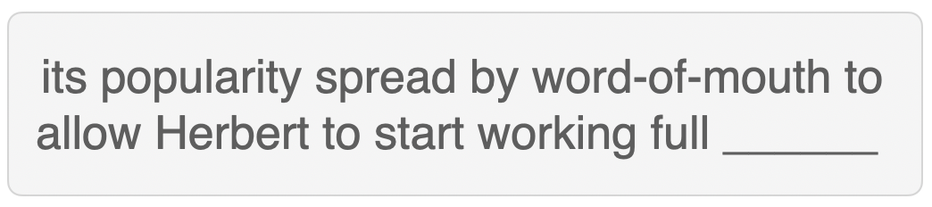
This distinction is important because LLMs encoded everything they know in their model parameters. While this makes sense for language information, it is inefficient for factual and world-knowledge information.
By including a retrieval method in the language model, the model can be much smaller. A neural database aids it with retrieving factual information it needs during text generation.
Training becomes fast with small language models, as training data memorization is reduced. Anyone can deploy these models on smaller and more affordable GPUs and tweak them as per need.
Mechanically, RETRO is an encoder-decoder model just like the original transformer. However, it augments the input sequence with the help of a retrieval database. The model finds the most probable sequences in the database and adds them to the input. RETRO works its magic to generate the output prediction.
Before we explore the model architecture, let’s dig deeper into the retrieval database.
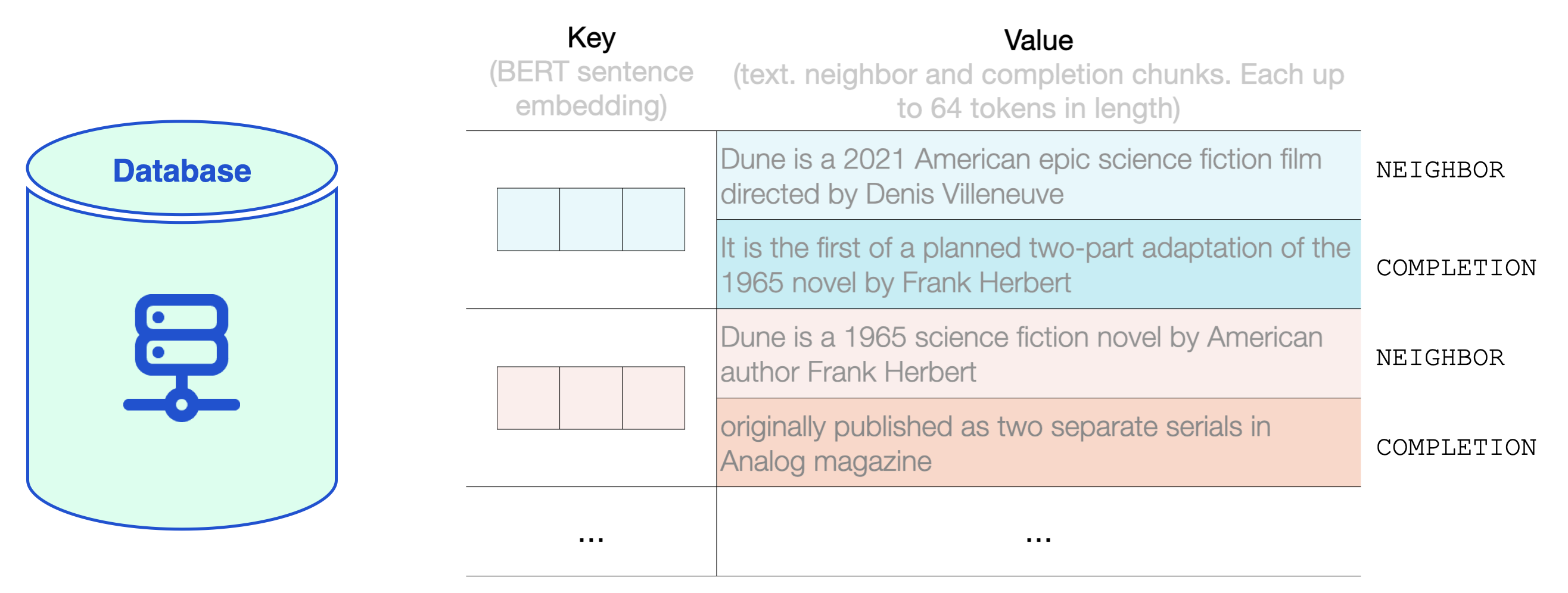
The database is a key-value store.
The key is a standard BERT sentence embedding.
The value is text in two parts:
Neighbor, which is used to compute the key
Completion, the continuation of the text in the original document.
RETRO’s database contains 2 trillion multi-lingual tokens based on the MassiveText dataset. Both the neighbor and completion chunks are at most 64 tokens long.
RETRO breaks the input prompt into multiple chunks. For simplicity, we’ll focus on how one chunk is augmented with retrieved text. The model, however, does this process for each chunk (except the first) in the input prompt.
Before hitting RETRO, the input prompt goes into BERT. The output contextualized vectors are then averaged to construct a sentence embedding vector. That vector is then used to query the database.
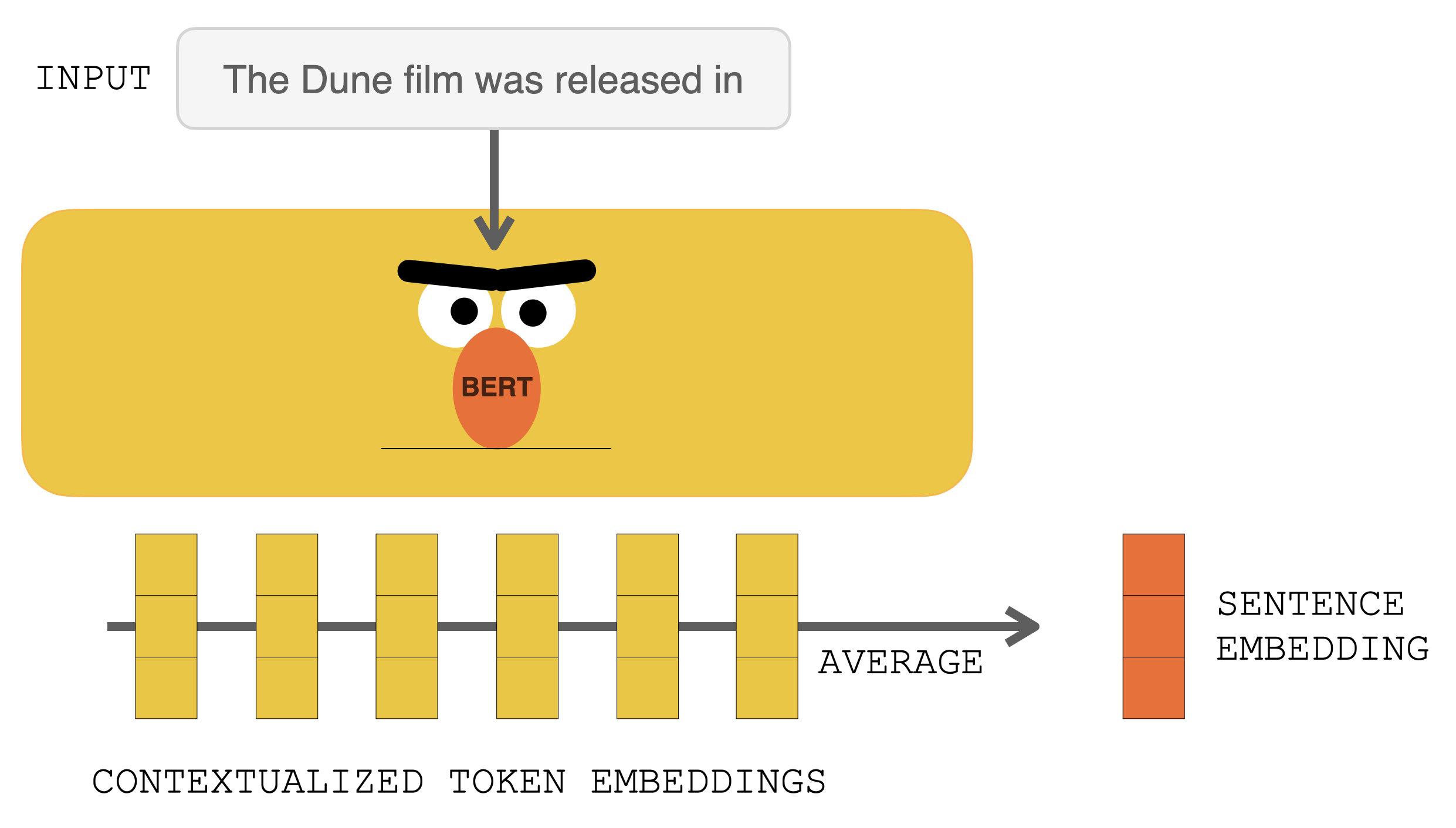
That sentence embedding is then used in an approximate nearest neighbor search (https://github.com/google-research/google-research/tree/master/scann).
The two nearest neighbors are retrieved, and their text becomes a part of the input into RETRO.
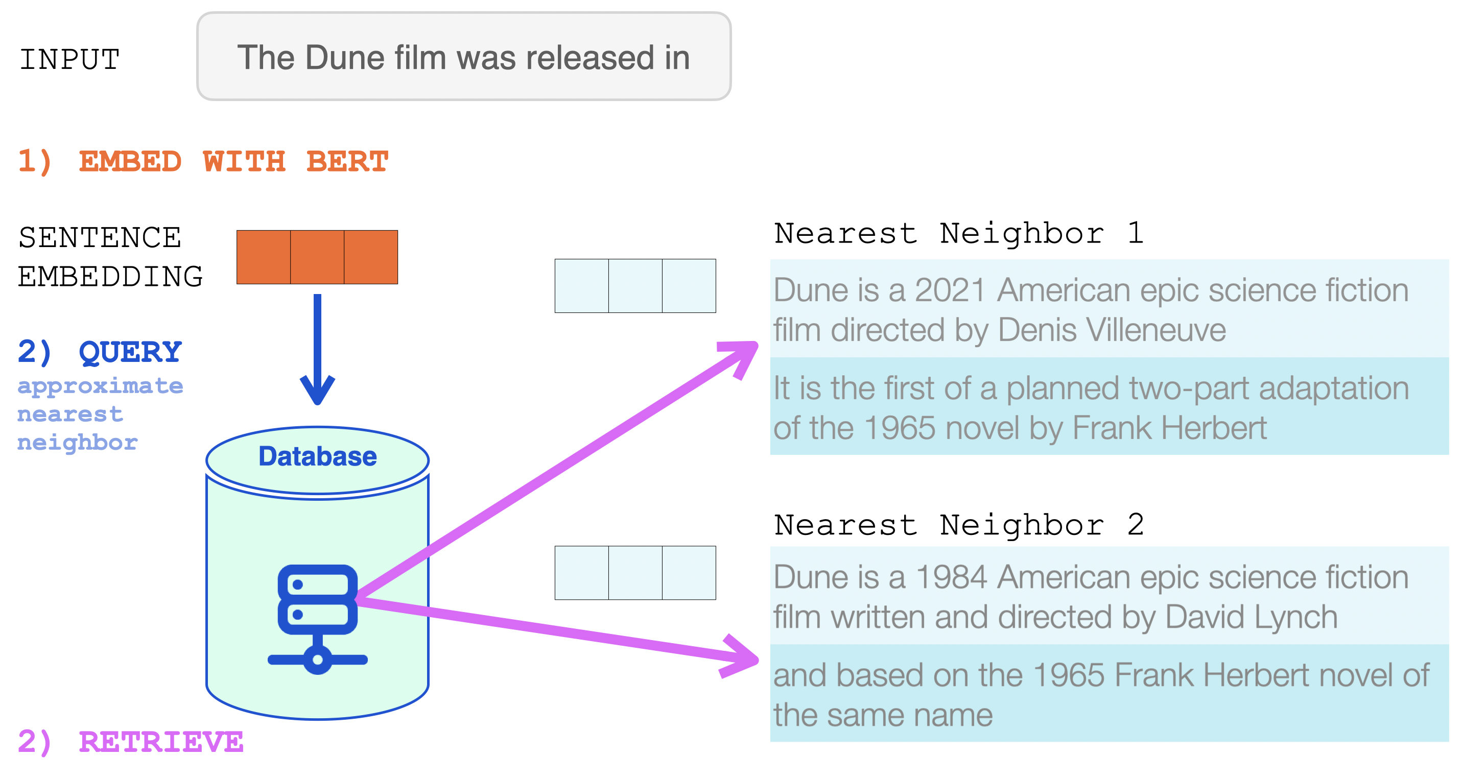
This is now the input to RETRO. The input prompt and its two nearest neighbors from the database (and their continuations).
From here, the Transformer and RETRO Blocks incorporate the information into their processing.
RETRO’s architecture is an encoder stack and a decoder stack.
The encoder is made up of standard Transformer encoder blocks (self-attention + FFNN). To my best understanding, Retro uses an encoder made up of two Transformer Encoder Blocks.
The decoder stack interleaves two kinds of decoder blocks:
Let’s start by looking at the encoder stack, which processes the retrieved neighbors, resulting in KEYS and VALUES matrices that will later be used for attention (see The Illustrated Transformer for a refresher).
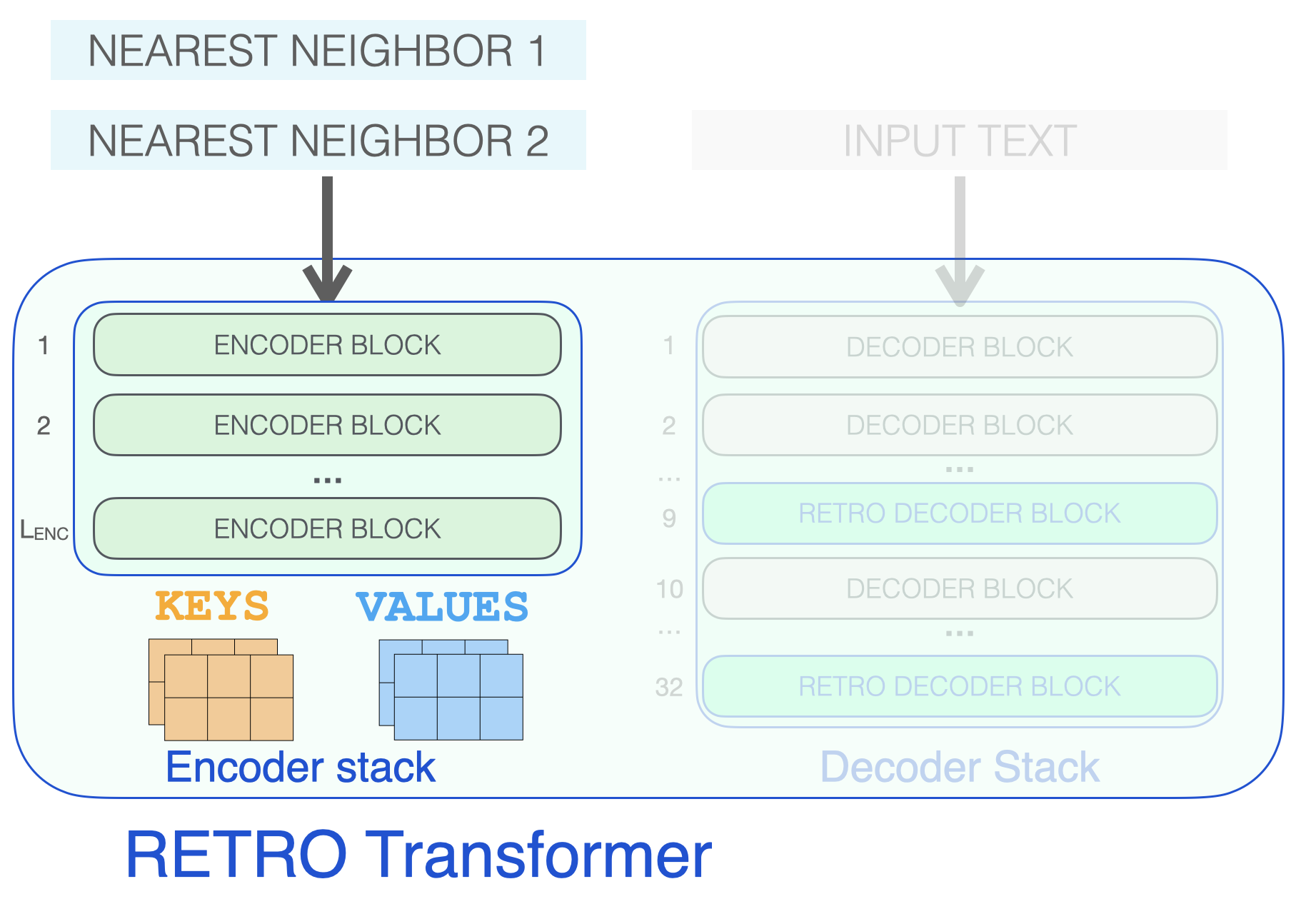
Decoder blocks process the input text just like a GPT would. It applies self-attention on the prompt token (causally, so only attending to previous tokens), then passes through a FFNN layer.
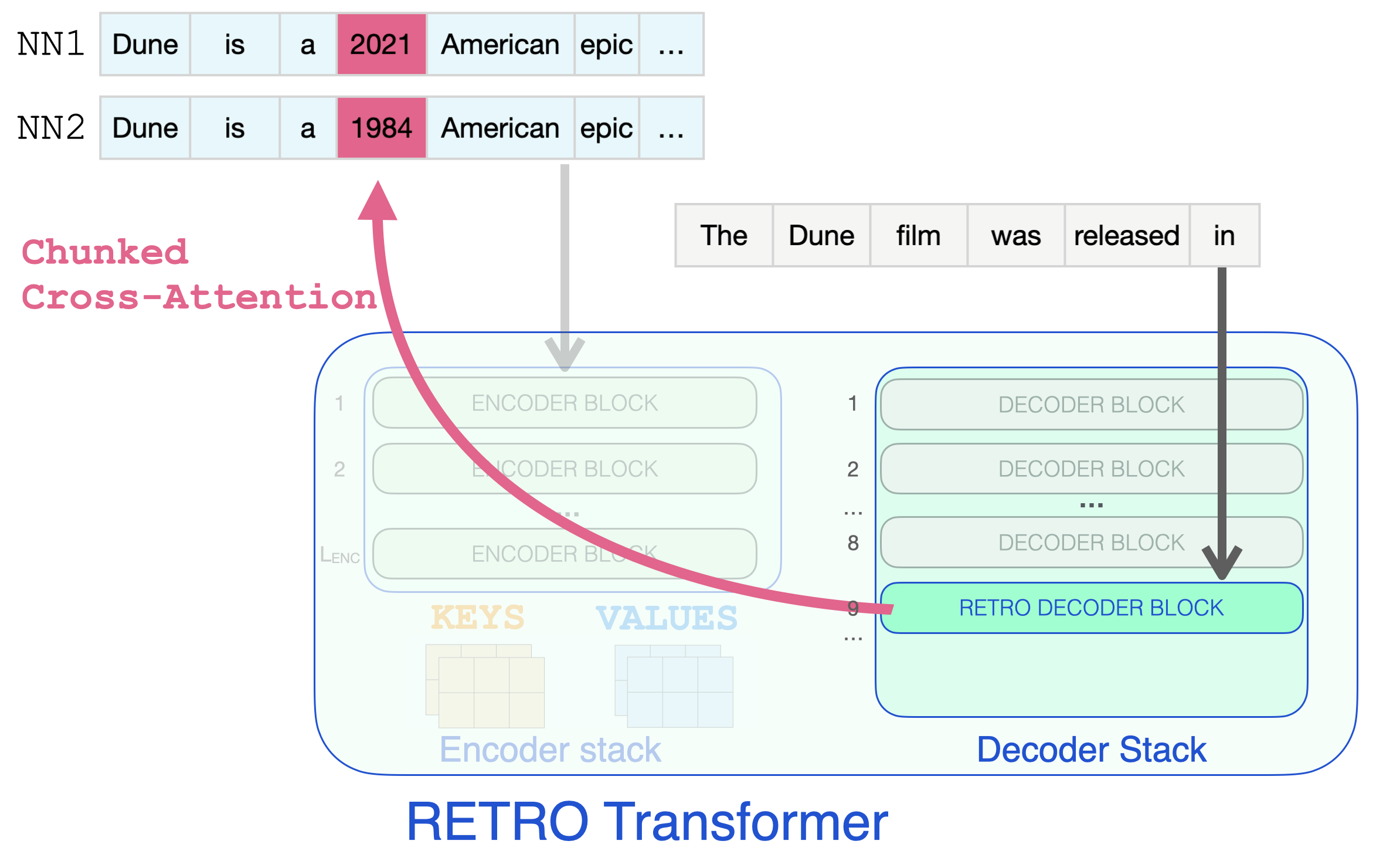
It’s only when a RETRO decoder is reached do we start to incorporate the retrieved information. Every third block starting from 9 is a RETRO block (that allows its input to attend to the neighbors). So layers 9, 12, 15…32 are RETRO blocks. (The two smaller Retro models, and the Retrofit models have these layers starting from the 6th instead of the 9th layer).
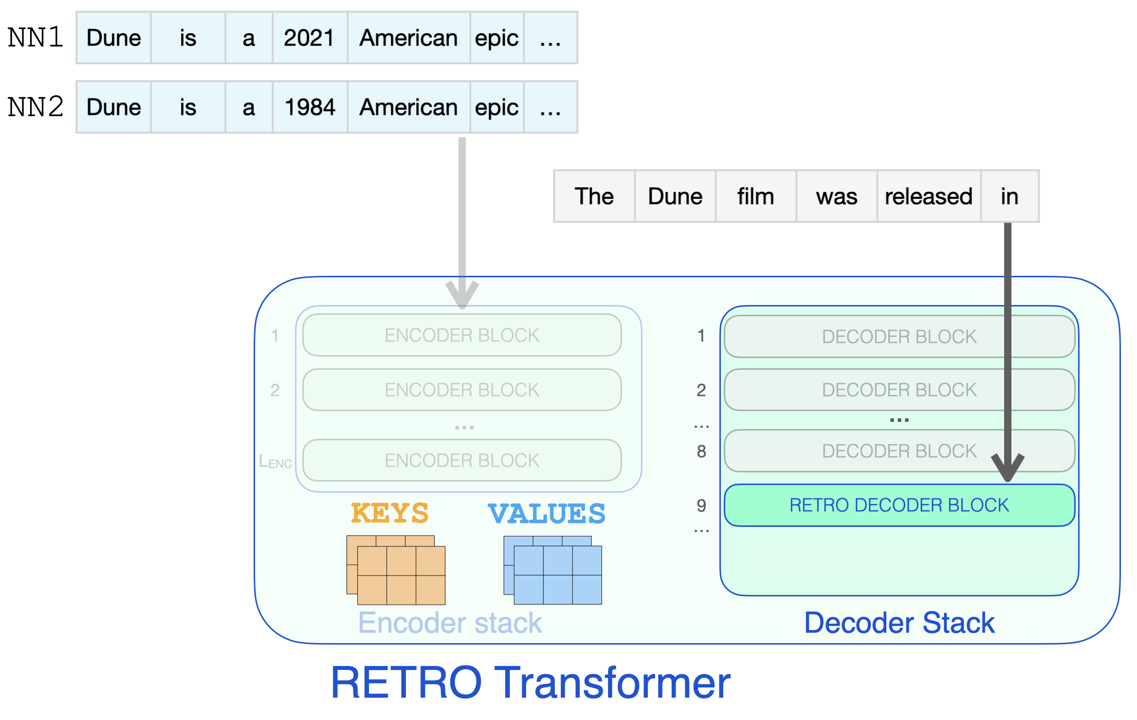
So effectively, this is the step where the retrieved information can glance at the dates it needs to complete the prompt.
Aiding language models with retrieval techniques has been an active area of research. Some of the previous work in the space includes:
Please post in this thread or reach out to me on Twitter for any corrections or feedback.
]]> 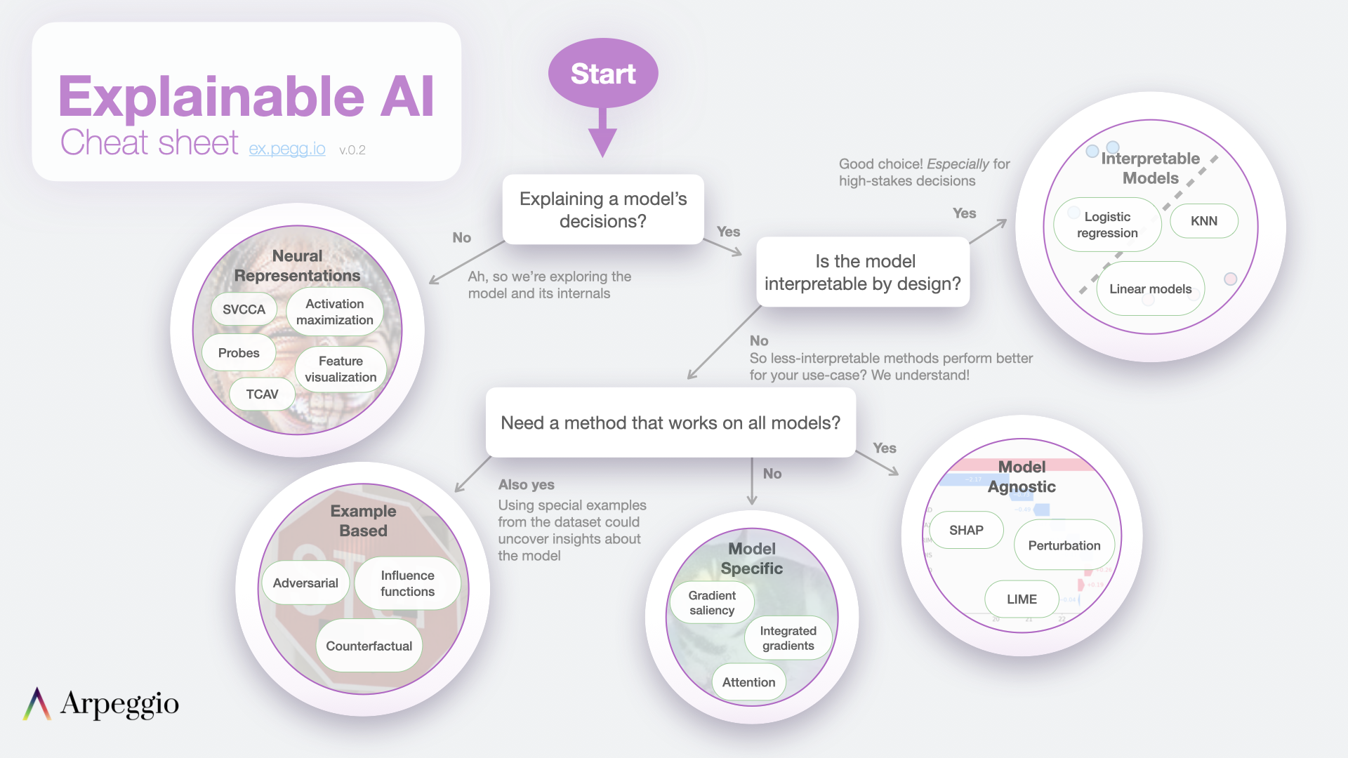
I introduce the cheat sheet in this brief video:
By visualizing the hidden state between a model's layers, we can get some clues as to the model's "thought process".
Part 2: Continuing the pursuit of making Transformer language models more transparent, this article showcases a collection of visualizations to uncover mechanics of language generation inside a pre-trained language model. These visualizations are all created using Ecco, the open-source package we're releasing
In the first part of this series, Interfaces for Explaining Transformer Language Models, we showcased interactive interfaces for input saliency and neuron activations. In this article, we will focus on the hidden state as it evolves from model layer to the next. By looking at the hidden states produced by every transformer decoder block, we aim to gleam information about how a language model arrived at a specific output token. This method is explored by Voita et al.. Nostalgebraist presents compelling visual treatments showcasing the evolution of token rankings, logit scores, and softmax probabilities for the evolving hidden state through the various layers of the model.
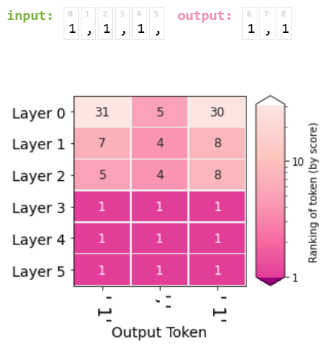
The following figure recaps how a transformer language model works. How the layers result in a final hidden state. And how that final state is then projected to the output vocabulary which results in a score assigned to each token in the model's vocabulary. We can see here the top scoring tokens when DistilGPT2 is fed the input sequence " 1, 1, ":
# Generate one token to complete this input string
output = lm.generate(" 1, 1, 1,", generate=1)

# Visualize
output.layer_predictions(position=6, layer=5)
Applying the same projection to internal hidden states of the model gives us a view of how the model's conviction for the output scoring developed over the processing of the inputs. This projection of internal hidden states gives us a sense of which layer contributed the most to elevating the scores (and hence ranking) of a certain potential output token.
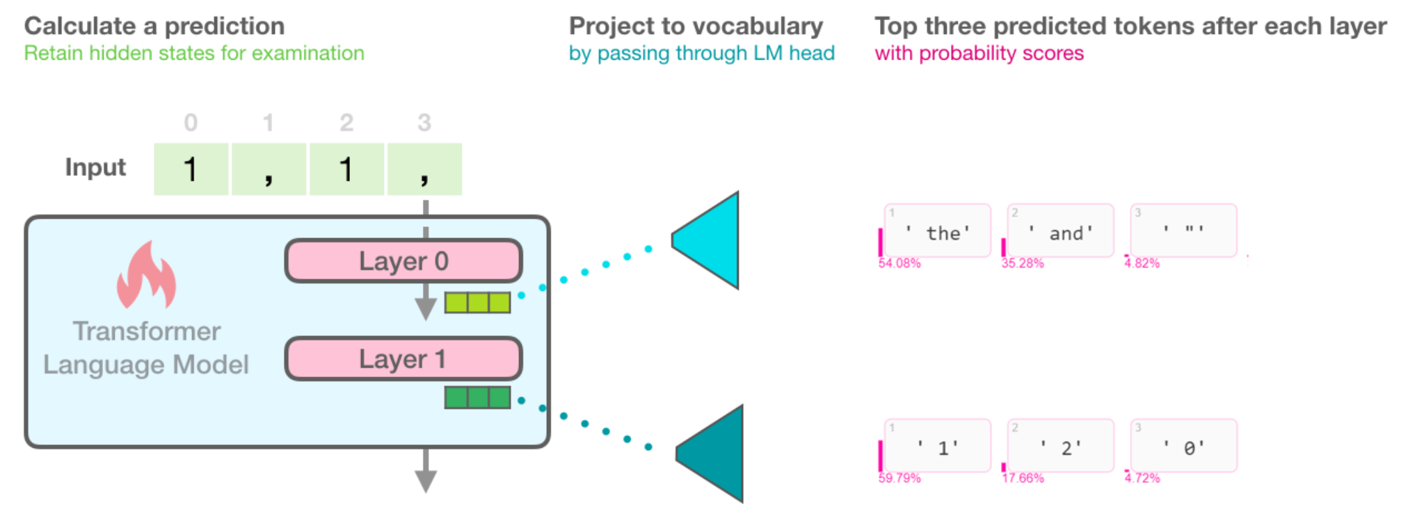
Viewing the evolution of the hidden states means that instead of looking only at the candidates output tokens from projecting the final model state, we can look at the top scoring tokens after projecting the hidden state resulting from each of the model's six layers.
This visualization is created using the same method above with omitting the 'layer' argument (which we set to the final layer in the previous example, layer #5):# Visualize the top scoring tokens after each layer
output.layer_predictions(position=6)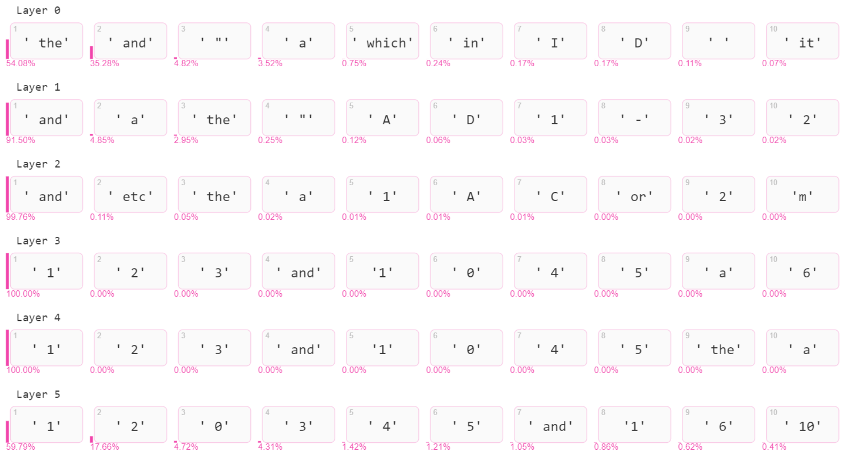
![]()
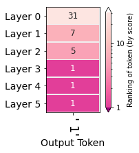
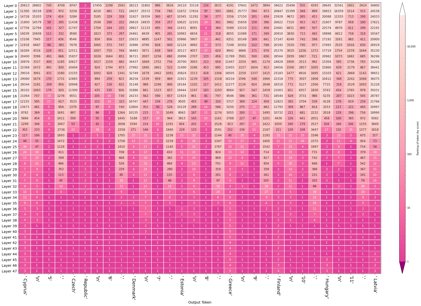
Another visual perspective on the evolving hidden states is to re-examine the hidden states after selecting an output token to see how the hidden state after each layer ranked that token. This is one of the many perspectives explored by Nostalgebraist and the one we think is a great first approach. In the figure on the side, we can see the ranking (out of +50,0000 tokens in the model's vocabulary) of the token ' 1' where each row indicates a layer's output.
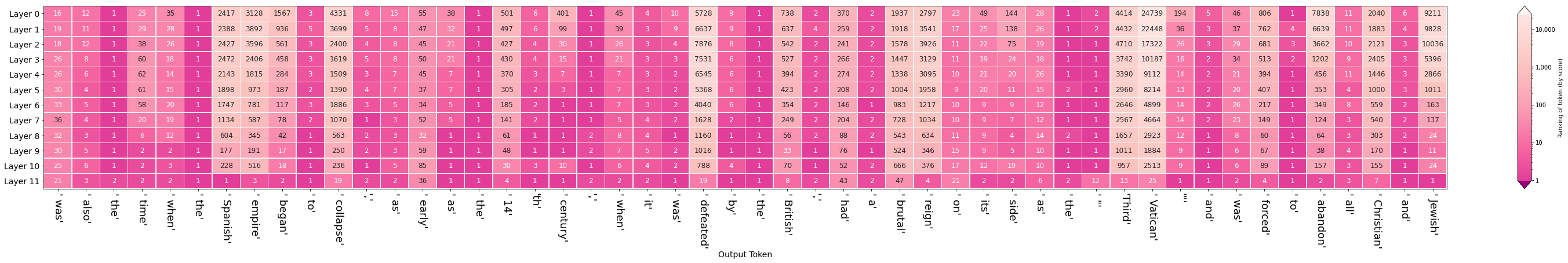
The same visualization can then be plotted for an entire generated sequence, where each column indicates a generation step (and its output token), and each row the ranking of the output token at each layer:
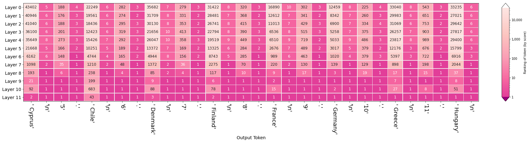
Let us demonstrate this visualization by presenting the following input to GPT2-Large:
Visualizaing the evolution of the hidden states sheds light on how various layers contribute to generating this sequence as we can see in the following figure:
![]()
We are not limited to watching the evolution of only one (the selected) token for a specific position. There are cases where we want to compare the rankings of multiple tokens in the same position regardless if the model selected them or not.
One such case is the number prediction task described by Linzen et al. which arises from the English language phenomenon of subject-verb agreement. In that task, we want to analyze the model's capacity to encode syntactic number (whether the subject we're addressing is singular or plural) and syntactic subjecthood (which subject in the sentence we're addressing).
Put simply, fill-in the blank. The only acceptable answers are 1) is 2) are:
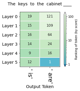
The keys to the cabinet ______
To answer correctly, one has to first determine whether we're describing the keys (possible subject #1) or the cabinet (possible subject #2). Having decided it is the keys, the second determination would be whether it is singular or plural.
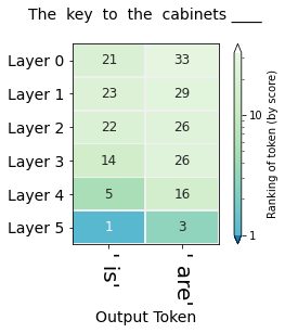
Contrast your answer for the first question with the following variation:
The key to the cabinets ______
The figures in this section visualize the hidden-state evolution of the tokens " is" and " are". The numbers in the cells are their ranking in the position of the blank (Both columns address the same position in the sequence, they're not subsequent positions as was the case in the previous visualization).
The first figure (showing the rankings for the sequence "The keys to the cabinet") raises the question of why do five layers fail the task and only the final layer sets the record straight. This is likely a similar effect to that observed in BERT of the final layer being the most task-specific. It is also worth investigating whether that capability of succeeding at the task is predominantly localized in Layer 5, or if the Layer is only the final expression in a circuit spanning multiple layers which is especially sensitive to subject-verb agreement.
This method can shed light on questions of bias and where they might emerge in a model. The following figures, for example, probe for the model's gender expectation associated with different professions:
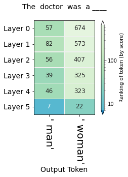
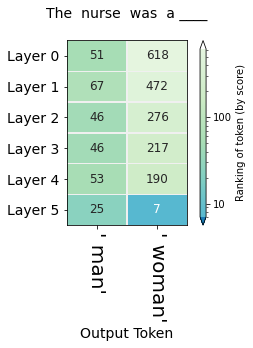
More systemaic and nuanced examination of bias in contextualized word embeddings (another term for the vectors we've been referring to as "hidden states") can be found in .
![]()


This article was vastly improved thanks to feedback on earlier drafts provided by Abdullah Almaatouq, Anfal Alatawi, Fahd Alhazmi, Hadeel Al-Negheimish, Isabelle Augenstein, Jasmijn Bastings, Najwa Alghamdi, Pepa Atanasova, and Sebastian Gehrmann.
Alammar, J. (2021). Finding the Words to Say: Hidden State Visualizations for Language Models [Blog post]. Retrieved from https://jalammar.github.io/hidden-states/
@misc{alammar2021hiddenstates,
  title={Finding the Words to Say: Hidden State Visualizations for Language Models},
  author={Alammar, J},
  year={2021},
  url={https://jalammar.github.io/hidden-states/}
}
Interfaces for exploring transformer language models by looking at input saliency and neuron activation.
The Transformer architecture has been powering a number of the recent advances in NLP. A breakdown of this architecture is provided here . Pre-trained language models based on the architecture, in both its auto-regressive (models that use their own output as input to next time-steps and that process tokens from left-to-right, like GPT2) and denoising (models trained by corrupting/masking the input and that process tokens bidirectionally, like BERT) variants continue to push the envelope in various tasks in NLP and, more recently, in computer vision. Our understanding of why these models work so well, however, still lags behind these developments.
This exposition series continues the pursuit to interpret and visualize the inner-workings of transformer-based language models. We illustrate how some key interpretability methods apply to transformer-based language models. This article focuses on auto-regressive models, but these methods are applicable to other architectures and tasks as well.
This is the first article in the series. In it, we present explorables and visualizations aiding the intuition of:
The next article addresses Hidden State Evolution across the layers of the model and what it may tell us about each layer's role.
In the language of Interpretable Machine Learning (IML) literature like Molnar et al., input saliency is a method that explains individual predictions. The latter two methods fall under the umbrella of "analyzing components of more complex models", and are better described as increasing the transparency of transformer models.
Moreover, this article is accompanied by reproducible notebooks and Ecco - an open source library to create similar interactive interfaces directly in Jupyter notebooks for GPT-based models from the HuggingFace transformers library.
If we're to impose the three components we're examining to explore the architecture of the transformer, it would look like the following figure.
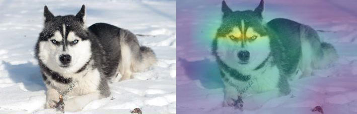
When a computer vision model classifies a picture as containing a husky, saliency maps can tell us whether the classification was made due to the visual properties of the animal itself, or because of the snow in the background. This is a method of attribution explaining the relationship between a model's output and inputs -- helping us detect errors and biases, and better understand the behavior of the system.
Multiple methods exist for assigning importance scores to the inputs of an NLP model. The literature is most often concerned with this application for classification tasks, rather than natural language generation. This article focuses on language generation. Our first interface calculates feature importance after each token is generated, and by hovering or tapping on an output token, imposes a saliency map on the tokens responsible for generating it.
The first example for this interface asks GPT2-XL for William Shakespeare's date of birth. The model is correctly able to produce the date (1564, but broken into two tokens: " 15" and "64", because the model's vocabulary does not include " 1564" as a single token). The interface shows the importance of each input token when generating each output token:
Our second example attempts to both probe a model's world knowledge, as well as to see if the model repeats the patterns in the text (simple patterns like the periods after numbers and like new lines, and slightly more involved patterns like completing a numbered list). The model used here is DistilGPT2.
This explorable shows a more detailed view that displays the attribution percentage for each token -- in case you need that precision.
Another example that we use illustratively in the rest of this article is one where we ask the model to complete a simple pattern:
It is also possible to use the interface to analyze the responses of a transformer-based conversational agent. In the following example, we pose an existential question to DiabloGPT:
![]()
Demonstrated above is scoring feature importance based on Gradients X Inputs-- a gradient-based saliency method shown by Atanasova et al. to perform well across various datasets for text classification in transformer models.
To illustrate how that works, let's first recall how the model generates the output token in each time step. In the following figure, we see how ① the language model's final hidden state is projected into the model's vocabulary resulting in a numeric score for each token in the model's vocabulary. Passing that scores vector through a softmax operation results in a probability score for each token. ② We proceed to select a token (e.g. select the highest-probability scoring token, or sample from the top scoring tokens) based on that vector.
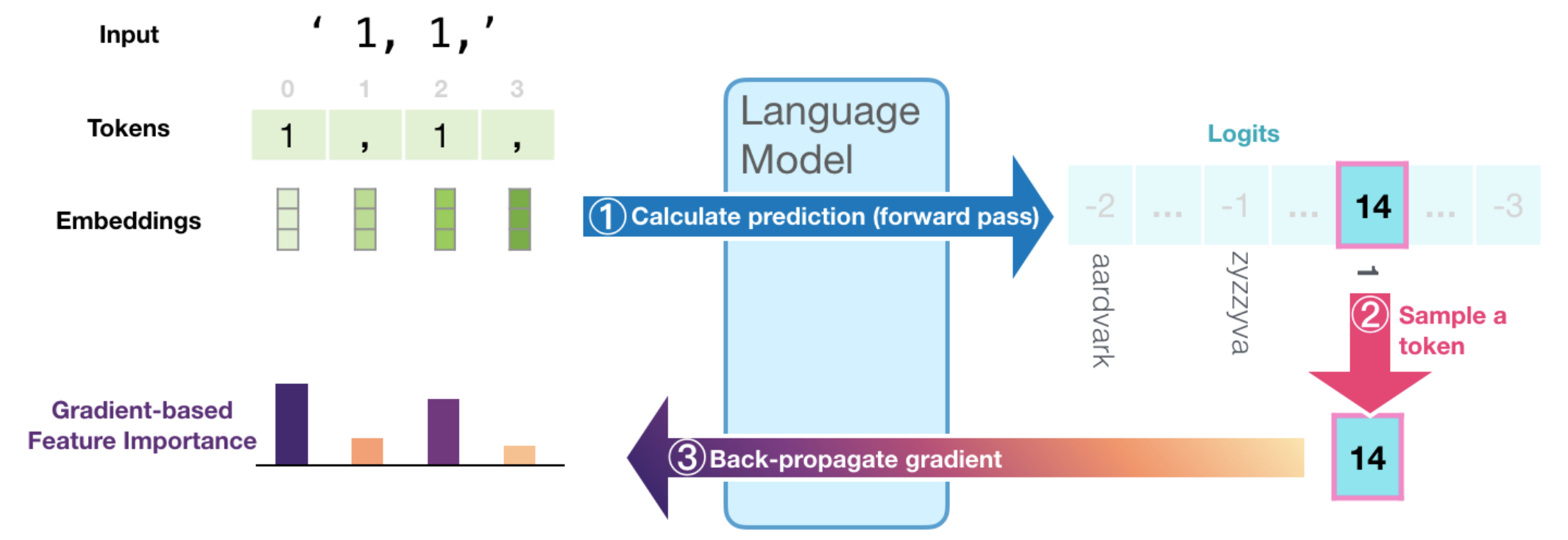
③ By calculating the gradient of the selected logit (before the softmax) with respect to the inputs by back-propagating it all the way back to the input tokens, we get a signal of how important each token was in the calculation resulting in this generated token. That assumption is based on the idea that the smallest change in the input token with the highest feature-importance value makes a large change in what the resulting output of the model would be.
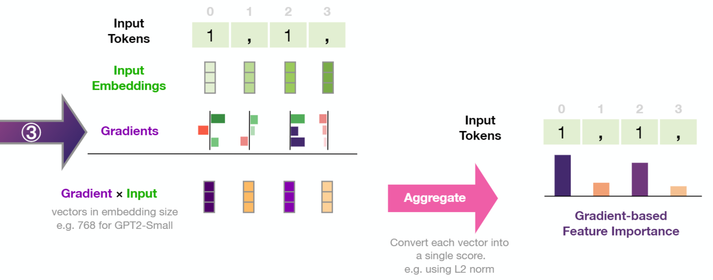
The resulting gradient vector per token is then multiplied by the input embedding of the respective token. Taking the L2 norm of the resulting vector results in the token's feature importance score. We then normalize the scores by dividing by the sum of these scores.
More formally, gradient × input is described as follows:
Where is the embedding vector of the input token at timestep i, and is the back-propagated gradient of the score of the selected token unpacked as follows:
This formalization is the one stated by Bastings et al. except the gradient and input vectors are multiplied element-wise. The resulting vector is then aggregated into a score via calculating the L2 norm as this was empirically shown in Atanasova et al. to perform better than other methods (like averaging).
The Feed Forward Neural Network (FFNN) sublayer is one of the two major components inside a transformer block (in addition to self-attention). It accounts for 66% of the parameters of a transformer block and thus provides a significant portion of the model's representational capacity. Previous work has examined neuron firings inside deep neural networks in both the NLP and computer vision domains. In this section we apply that examination to transformer-based language models.
To guide our neuron examination, let's present our model with the input "1, 2, 3" in hopes it would echo the comma/number alteration, yet also keep incrementing the numbers.
It succeeds.
By using the methods we'll discuss in Article #2 (following the lead of nostalgebraist), we can produce a graphic that exposes the probabilities of output tokens after each layer in the model. This looks at the hidden state after each layer, and displays the ranking of the ultimately produced output token in that layer.
For example, in the first step, the model produced the token " 4". The first column tells us about that process. The bottom most cell in that column shows that the token " 4" was ranked #1 in probability after the last layer. Meaning that the last layer (and thus the model) gave it the highest probability score. The cells above indicate the ranking of the token " 4" after each layer.
By looking at the hidden states, we observe that the model gathers confidence about the two patterns of the output sequence (the commas, and the ascending numbers) at different layers.
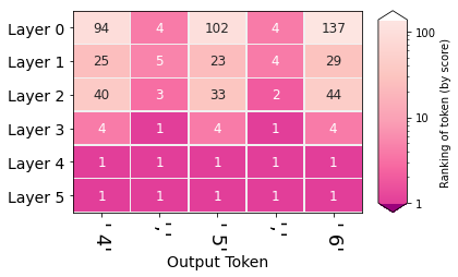
What happens at Layer 4 which makes the model elevate the digits (4, 5, 6) to the top of the probability distribution?
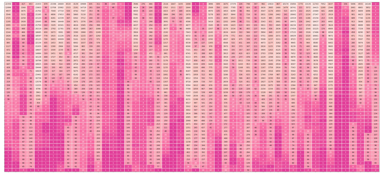
We can plot the activations of the neurons in layer 4 to get a sense of neuron activity. That is what the first of the following three figures shows.
It is difficult, however, to gain any interpretation from looking at activations during one forward pass through the model.
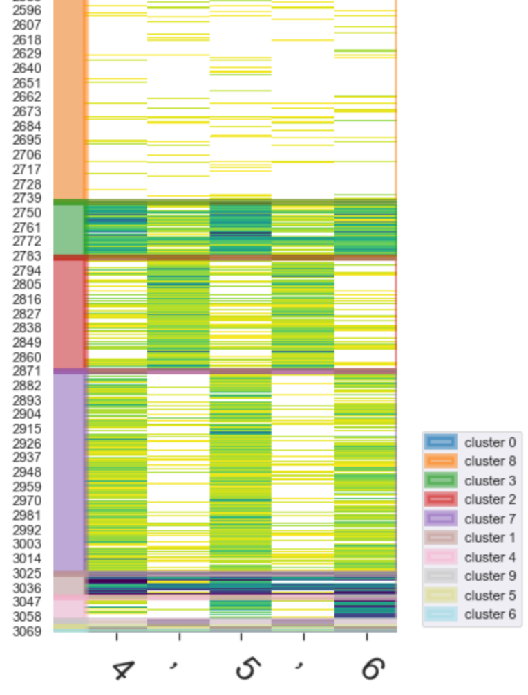
The figures below show neuron activations while five tokens are generated (' 4 , 5 , 6'). To get around the sparsity of the firings, we may wish to cluster the firings, which is what the subsequent figure shows.
|
Each row is a neuron. Only neurons with positive activation are colored. The darker they are, the more intense the firing. |
|
Each row corresponds to a neuron in the feedforward neural network of layer #4. Each column is that neuron's status when a token was generated (namely, the token at the top of the figure). A view of the first 400 neurons shows how sparse the activations usually are (out of the 3072 neurons in the FFNN layer in DistilGPT2). |
|
Clustering Neurons by Activation Values To locate the signal, the neurons are clustered (using kmeans on the activation values) to reveal the firing pattern. We notice:
|
If visualized and examined properly, neuron firings can reveal the complementary and compositional roles that can be played by individual neurons, and groups of neurons.
Even after clustering, looking directly at activations is a crude and noisy affair. As presented in Olah et al., we are better off reducing the dimensionality using a matrix decomposition method. We follow the authors' suggestion to use Non-negative Matrix Factorization (NMF) as a natural candidate for reducing the dimensionality into groups that are potentially individually more interpretable. Our first experiments were with Principal Component Analysis (PCA), but NMF is a better approach because it's difficult to interpret the negative values in a PCA component of neuron firings.
By first capturing the activations of the neurons in FFNN layers of the model, and then decomposing them into a more manageable number of factors (using) using NMF, we are able to shed light on how various neurons contributed towards each generated token.
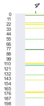
The simplest approach is to break down the activations into two factors. In our next interface, we have the model generate thirty tokens, decompose the activations into two factors, and highlight each token with the factor with the highest activation when that token was generated:
This interface is capable of compressing a lot of data that showcase the excitement levels of factors composed of groups of neurons. The sparklines on the left give a snapshot of the excitement level of each factor across the entire sequence. Interacting with the sparklines (by hovering with a mouse or tapping on touchscreens) displays the activation of the factor on the tokens in the sequence on the right.
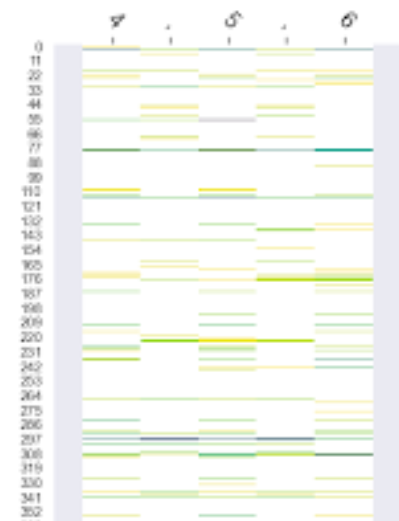
We can see that decomposing activations into two factors resulted in factors that correspond with the alternating patterns we're analyzing (commas, and incremented numbers). We can increase the resolution of the factor analysis by increasing the number of factors. The following figure decomposes the same activations into five factors.
We can start extending this to input sequences with more content, like the list of EU countries:
Another example, of how DistilGPT2 reacts to XML, shows a clear distinction of factors attending to different components of the syntax. This time we are breaking down the activations into ten components:
This interface is a good companion for hidden state examinations which can highlight a specific layer of interest, and using this interface we can focus our analysis on that layer of interest. It is straight-forward to apply this method to specific layers of interest. Hidden-state evolution diagrams, for example, indicate that layer #0 does a lot of heavy lifting as it often tends to shortlist the tokens that make it to the top of the probability distribution. The following figure showcases ten factors applied to the activations of layer 0 in response to a passage by Fyodor Dostoyevsky:
We can crank up the resolution by increasing the number of factors. Increasing this to eighteen factors starts to reveal factors that light up in response to adverbs, and other factors that light up in response to partial tokens. Increase the number of factors more and you'll start to identify factors that light up in response to specific words ("nothing" and "man" seem especially provocative to the layer).
The explorables above show the factors resulting from decomposing the matrix holding the activations values of FFNN neurons using Non-negative Matrix Factorization. The following figure sheds light on how that is done:
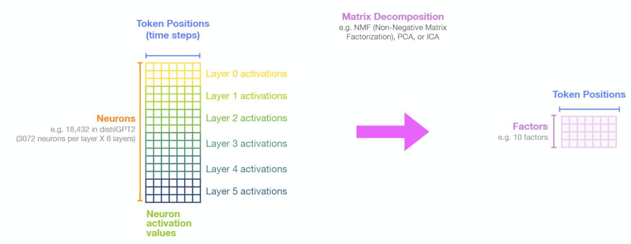
Beyond dimensionality reduction, Non-negative Matrix Factorization can reveal underlying common behaviour of groups of neurons. It can be used to analyze the entire network, a single layer, or groups of layers.
![]()
This concludes the first article in the series. Be sure to click on the notebooks and play with Ecco! I would love your feedback on this article, series, and on Ecco in this thread. If you find interesting factors or neurons, feel free to post them there as well. I welcome all feedback!
This article was vastly improved thanks to feedback on earlier drafts provided by Abdullah Almaatouq, Ahmad Alwosheel, Anfal Alatawi, Christopher Olah, Fahd Alhazmi, Hadeel Al-Negheimish, Isabelle Augenstein, Jasmijn Bastings, Najla Alariefy, Najwa Alghamdi, Pepa Atanasova, and Sebastian Gehrmann.
Alammar, J. (2020). Interfaces for Explaining Transformer Language Models
[Blog post]. Retrieved from https://jalammar.github.io/explaining-transformers/
@misc{alammar2020explaining,
  title={Interfaces for Explaining Transformer Language Models},
  author={Alammar, J},
  year={2020},
  url={https://jalammar.github.io/explaining-transformers/}
}
The tech world is abuzz with GPT3 hype. Massive language models (like GPT3) are starting to surprise us with their abilities. While not yet completely reliable for most businesses to put in front of their customers, these models are showing sparks of cleverness that are sure to accelerate the march of automation and the possibilities of intelligent computer systems. Let’s remove the aura of mystery around GPT3 and learn how it’s trained and how it works.
A trained language model generates text.
We can optionally pass it some text as input, which influences its output.
The output is generated from what the model “learned” during its training period where it scanned vast amounts of text.
Training is the process of exposing the model to lots of text. That process has been completed. All the experiments you see now are from that one trained model. It was estimated to cost 355 GPU years and cost $4.6m.
The dataset of 300 billion tokens of text is used to generate training examples for the model. For example, these are three training examples generated from the one sentence at the top.
You can see how you can slide a window across all the text and make lots of examples.
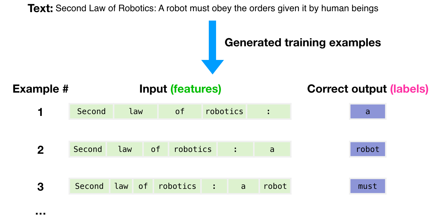
The model is presented with an example. We only show it the features and ask it to predict the next word.
The model’s prediction will be wrong. We calculate the error in its prediction and update the model so next time it makes a better prediction.
Repeat millions of times
Now let’s look at these same steps with a bit more detail.
GPT3 actually generates output one token at a time (let’s assume a token is a word for now).
Please note: This is a description of how GPT-3 works and not a discussion of what is novel about it (which is mainly the ridiculously large scale). The architecture is a transformer decoder model based on this paper https://arxiv.org/pdf/1801.10198.pdf
GPT3 is MASSIVE. It encodes what it learns from training in 175 billion numbers (called parameters). These numbers are used to calculate which token to generate at each run.
The untrained model starts with random parameters. Training finds values that lead to better predictions.
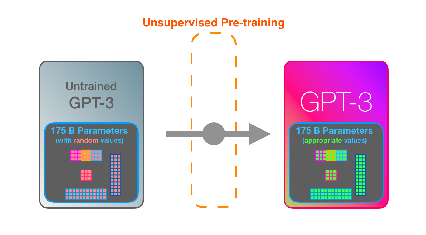
These numbers are part of hundreds of matrices inside the model. Prediction is mostly a lot of matrix multiplication.
In my Intro to AI on YouTube, I showed a simple ML model with one parameter. A good start to unpack this 175B monstrosity.
To shed light on how these parameters are distributed and used, we’ll need to open the model and look inside.
GPT3 is 2048 tokens wide. That is its “context window”. That means it has 2048 tracks along which tokens are processed.
Let’s follow the purple track. How does a system process the word “robotics” and produce “A”?
High-level steps:
The important calculations of the GPT3 occur inside its stack of 96 transformer decoder layers.
See all these layers? This is the “depth” in “deep learning”.
Each of these layers has its own 1.8B parameter to make its calculations. That is where the “magic” happens. This is a high-level view of that process:
You can see a detailed explanation of everything inside the decoder in my blog post The Illustrated GPT2.
The difference with GPT3 is the alternating dense and sparse self-attention layers.
This is an X-ray of an input and response (“Okay human”) within GPT3. Notice how every token flows through the entire layer stack. We don’t care about the output of the first words. When the input is done, we start caring about the output. We feed every word back into the model.
In the React code generation example, the description would be the input prompt (in green), in addition to a couple of examples of description=>code, I believe. And the react code would be generated like the pink tokens here token after token.
My assumption is that the priming examples and the description are appended as input, with specific tokens separating examples and the results. Then fed into the model.
It’s impressive that this works like this. Because you just wait until fine-tuning is rolled out for the GPT3. The possibilities will be even more amazing.
Fine-tuning actually updates the model’s weights to make the model better at a certain task.