
Visualizing A Neural Machine Translation Model (Mechanics of Seq2seq Models With Attention)
Translations: Chinese (Simplified), French, Japanese, Korean, Persian, Russian, Turkish, Uzbek
Watch: MIT’s Deep Learning State of the Art lecture referencing this post
May 25th update: New graphics (RNN animation, word embedding graph), color coding, elaborated on the final attention example.
Note: The animations below are videos. Touch or hover on them (if you’re using a mouse) to get play controls so you can pause if needed.
Sequence-to-sequence models are deep learning models that have achieved a lot of success in tasks like machine translation, text summarization, and image captioning. Google Translate started using such a model in production in late 2016. These models are explained in the two pioneering papers (Sutskever et al., 2014, Cho et al., 2014).
I found, however, that understanding the model well enough to implement it requires unraveling a series of concepts that build on top of each other. I thought that a bunch of these ideas would be more accessible if expressed visually. That’s what I aim to do in this post. You’ll need some previous understanding of deep learning to get through this post. I hope it can be a useful companion to reading the papers mentioned above (and the attention papers linked later in the post).
A sequence-to-sequence model is a model that takes a sequence of items (words, letters, features of an images…etc) and outputs another sequence of items. A trained model would work like this:
In neural machine translation, a sequence is a series of words, processed one after another. The output is, likewise, a series of words:
Looking under the hood
Under the hood, the model is composed of an encoder and a decoder.
The encoder processes each item in the input sequence, it compiles the information it captures into a vector (called the context). After processing the entire input sequence, the encoder sends the context over to the decoder, which begins producing the output sequence item by item.
The same applies in the case of machine translation.
The context is a vector (an array of numbers, basically) in the case of machine translation. The encoder and decoder tend to both be recurrent neural networks (Be sure to check out Luis Serrano’s A friendly introduction to Recurrent Neural Networks for an intro to RNNs).
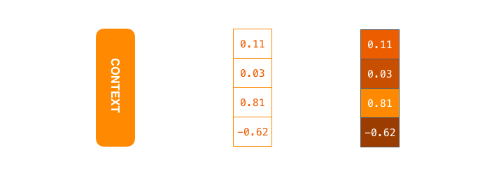 The context is a vector of floats. Later in this post we will visualize vectors in color by assigning brighter colors to the cells with higher values.
You can set the size of the context vector when you set up your model. It is basically the number of hidden units in the encoder RNN. These visualizations show a vector of size 4, but in real world applications the context vector would be of a size like 256, 512, or 1024.
By design, a RNN takes two inputs at each time step: an input (in the case of the encoder, one word from the input sentence), and a hidden state. The word, however, needs to be represented by a vector. To transform a word into a vector, we turn to the class of methods called “word embedding” algorithms. These turn words into vector spaces that capture a lot of the meaning/semantic information of the words (e.g. king - man + woman = queen).
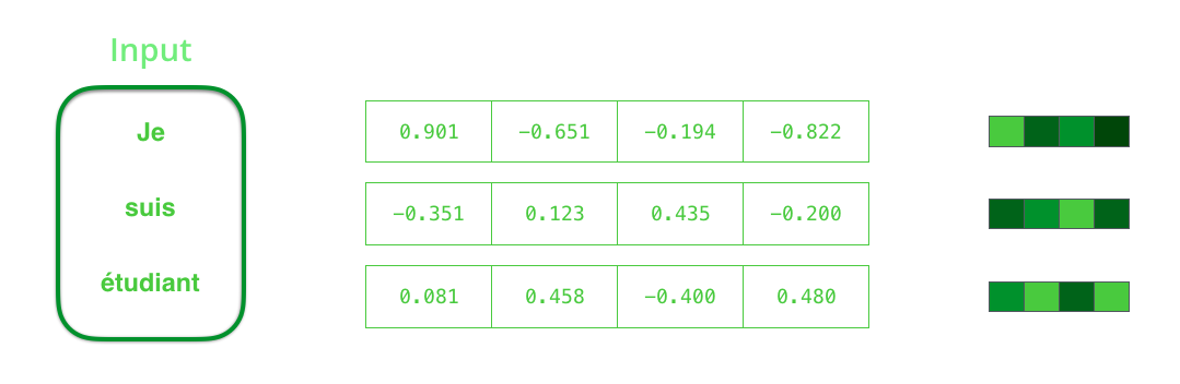 We need to turn the input words into vectors before processing them. That transformation is done using a word embedding algorithm. We can use pre-trained embeddings or train our own embedding on our dataset. Embedding vectors of size 200 or 300 are typical, we're showing a vector of size four for simplicity.
Now that we’ve introduced our main vectors/tensors, let’s recap the mechanics of an RNN and establish a visual language to describe these models:
The next RNN step takes the second input vector and hidden state #1 to create the output of that time step. Later in the post, we’ll use an animation like this to describe the vectors inside a neural machine translation model.
In the following visualization, each pulse for the encoder or decoder is that RNN processing its inputs and generating an output for that time step. Since the encoder and decoder are both RNNs, each time step one of the RNNs does some processing, it updates its hidden state based on its inputs and previous inputs it has seen.
Let’s look at the hidden states for the encoder. Notice how the last hidden state is actually the context we pass along to the decoder.
The decoder also maintains a hidden state that it passes from one time step to the next. We just didn’t visualize it in this graphic because we’re concerned with the major parts of the model for now.
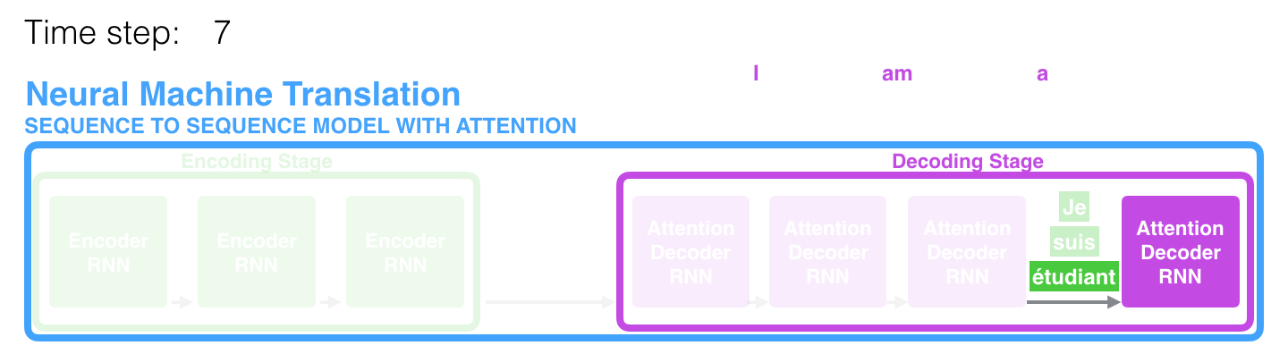
Let’s now look at another way to visualize a sequence-to-sequence model. This animation will make it easier to understand the static graphics that describe these models. This is called an “unrolled” view where instead of showing the one decoder, we show a copy of it for each time step. This way we can look at the inputs and outputs of each time step.
Let’s Pay Attention Now
The context vector turned out to be a bottleneck for these types of models. It made it challenging for the models to deal with long sentences. A solution was proposed in Bahdanau et al., 2014 and Luong et al., 2015. These papers introduced and refined a technique called “Attention”, which highly improved the quality of machine translation systems. Attention allows the model to focus on the relevant parts of the input sequence as needed.
Let’s continue looking at attention models at this high level of abstraction. An attention model differs from a classic sequence-to-sequence model in two main ways:
First, the encoder passes a lot more data to the decoder. Instead of passing the last hidden state of the encoding stage, the encoder passes all the hidden states to the decoder:
Second, an attention decoder does an extra step before producing its output. In order to focus on the parts of the input that are relevant to this decoding time step, the decoder does the following:
- Look at the set of encoder hidden states it received – each encoder hidden state is most associated with a certain word in the input sentence
- Give each hidden state a score (let’s ignore how the scoring is done for now)
- Multiply each hidden state by its softmaxed score, thus amplifying hidden states with high scores, and drowning out hidden states with low scores
This scoring exercise is done at each time step on the decoder side.
Let us now bring the whole thing together in the following visualization and look at how the attention process works:
- The attention decoder RNN takes in the embedding of the token, and an initial decoder hidden state.
- The RNN processes its inputs, producing an output and a new hidden state vector (h4). The output is discarded.
- Attention Step: We use the encoder hidden states and the h4 vector to calculate a context vector (C4) for this time step.
- We concatenate h4 and C4 into one vector.
- We pass this vector through a feedforward neural network (one trained jointly with the model).
- The output of the feedforward neural networks indicates the output word of this time step.
- Repeat for the next time steps
This is another way to look at which part of the input sentence we’re paying attention to at each decoding step:
Note that the model isn’t just mindless aligning the first word at the output with the first word from the input. It actually learned from the training phase how to align words in that language pair (French and English in our example). An example for how precise this mechanism can be comes from the attention papers listed above:
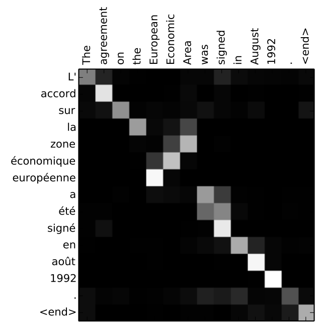 You can see how the model paid attention correctly when outputing "European Economic Area". In French, the order of these words is reversed ("européenne économique zone") as compared to English. Every other word in the sentence is in similar order.
If you feel you’re ready to learn the implementation, be sure to check TensorFlow’s Neural Machine Translation (seq2seq) Tutorial.
I hope you’ve found this useful. These visuals are early iterations of a lesson on attention that is part of the Udacity Natural Language Processing Nanodegree Program. We go into more details in the lesson, including discussing applications and touching on more recent attention methods like the Transformer model from Attention Is All You Need.
Check out the trailer of the NLP Nanodegree Program:
I’ve also created a few lessons as a part of Udacity’s Machine Learning Nanodegree Program. The lessons I’ve created cover Unsupervised Learning, as well as a jupyter notebook on movie recommendations using collaborative filtering.
I’d love any feedback you may have. Please reach me at @JayAlammmar.
