Finding the Words to Say: Hidden State Visualizations for Language Models
By visualizing the hidden state between a model's layers, we can get some clues as to the model's "thought process".
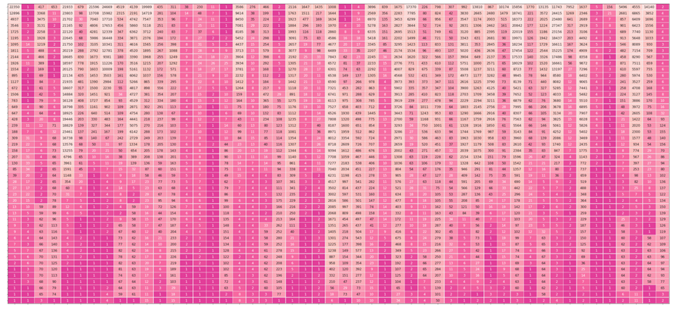
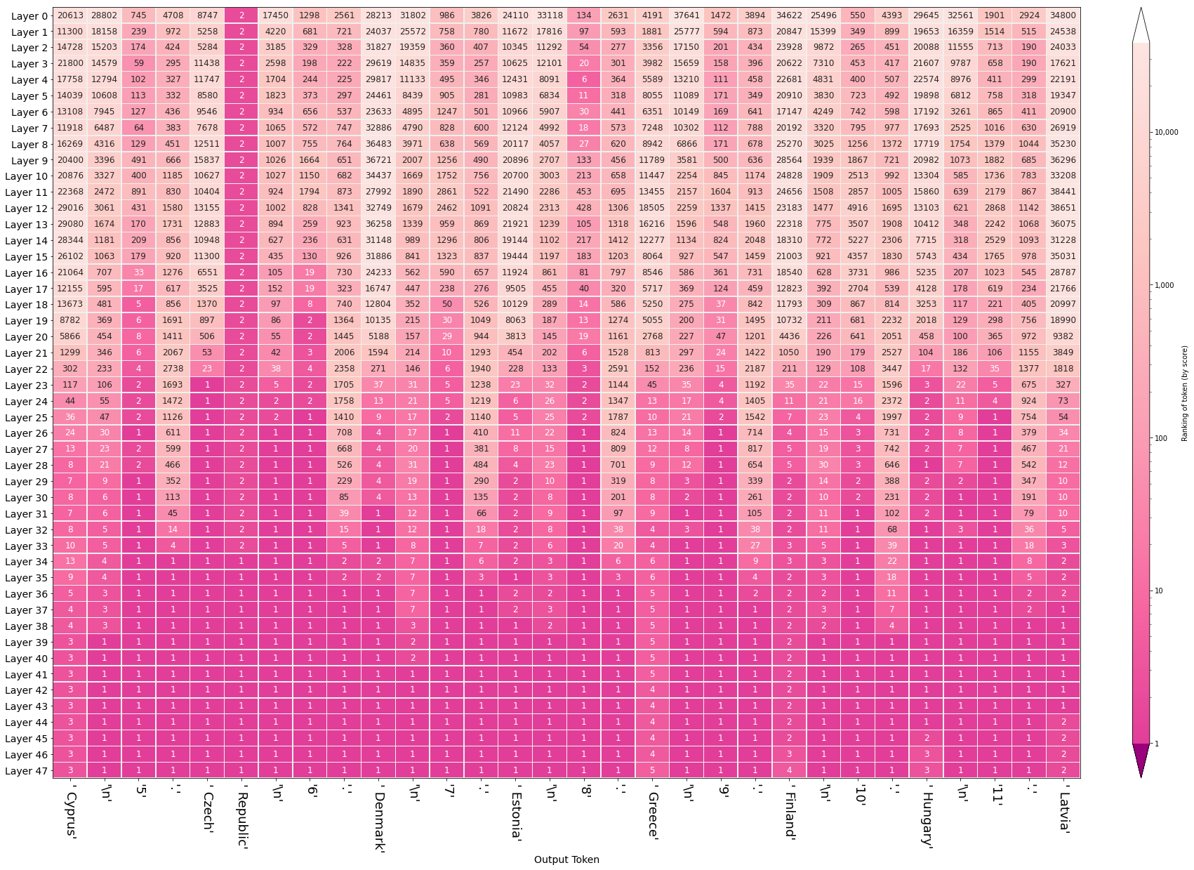
After a language model generates a sentence, we can visualize a view of how the model came by each word (column). Each row is a model layer. The value and color indicate the ranking of the output token at that layer. The darker the color, the higher the ranking. Layer 0 is at the top. Layer 47 is at the bottom.
Model:GPT2-XL
Part 2: Continuing the pursuit of making Transformer language models more transparent, this article showcases a collection of visualizations to uncover mechanics of language generation inside a pre-trained language model. These visualizations are all created using Ecco, the open-source package we're releasing
In the first part of this series, Interfaces for Explaining Transformer Language Models, we showcased interactive interfaces for input saliency and neuron activations. In this article, we will focus on the hidden state as it evolves from model layer to the next. By looking at the hidden states produced by every transformer decoder block, we aim to gleam information about how a language model arrived at a specific output token. This method is explored by Voita et al.. Nostalgebraist presents compelling visual treatments showcasing the evolution of token rankings, logit scores, and softmax probabilities for the evolving hidden state through the various layers of the model.
Recap: Transformer Hidden States
The following figure recaps how a transformer language model works. How the layers result in a final hidden state. And how that final state is then projected to the output vocabulary which results in a score assigned to each token in the model's vocabulary. We can see here the top scoring tokens when DistilGPT2 is fed the input sequence " 1, 1, ":
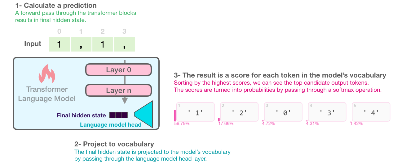
This figure shows how the model arrives at the top five output token candidates and their probability scores. This shows us that at the final layer, the model is 59% sure the next token is ' 1', and that would be chosen as the output token by greedy decoding. Other probable outputs include ' 2' with 18% probability (maybe we are counting) and ' 0' with 5% probability (maybe we are counting down).
# Generate one token to complete this input string
output = lm.generate(" 1, 1, 1,", generate=1)

# Visualize
output.layer_predictions(position=6, layer=5)
Scores after each layer
Applying the same projection to internal hidden states of the model gives us a view of how the model's conviction for the output scoring developed over the processing of the inputs. This projection of internal hidden states gives us a sense of which layer contributed the most to elevating the scores (and hence ranking) of a certain potential output token.
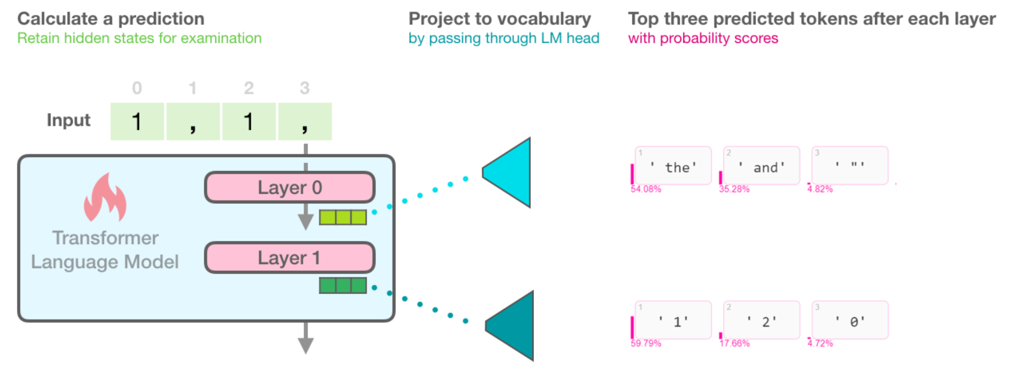
Viewing the evolution of the hidden states means that instead of looking only at the candidates output tokens from projecting the final model state, we can look at the top scoring tokens after projecting the hidden state resulting from each of the model's six layers.
This visualization is created using the same method above with omitting the 'layer' argument (which we set to the final layer in the previous example, layer #5):# Visualize the top scoring tokens after each layer
output.layer_predictions(position=6)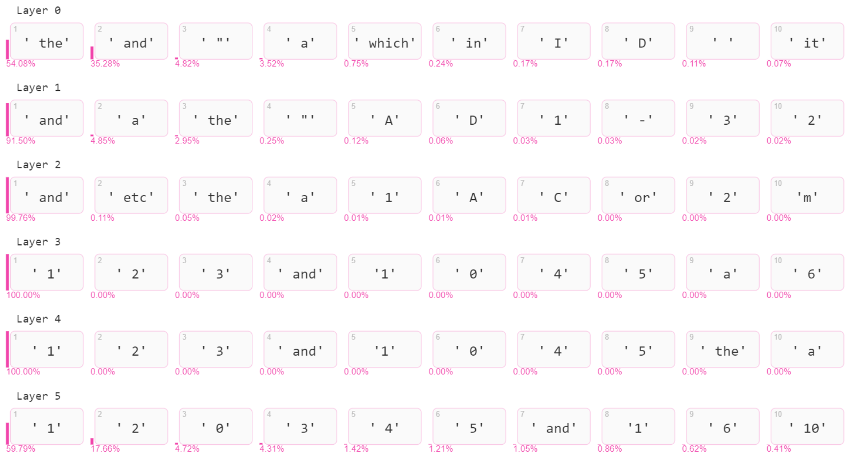
Each row shows the top ten predicted tokens obtained by projecting each hidden state to the output vocabulary. The probability scores are shown in pink (obtained by passing logit scores through softmax). We can see that Layer 0 has no digits in its top ten predictions. Layer 1 gives the token ' 1' a 0.03%, probability which, while low, still ranks the token as the seventh highest ranking token. Subsequent layers keep elevating the probability and ranking of ' 1', until the final layer injects a bit more caution by reducing the probability from 100% to ~60%, still retaining the token as the highest ranked in the model's output.
Note: This figure is incorrect in showing 0 probability assigned to some tokens due to rounding. The current version of Ecco fixes this by showing '<0.01%'.
Evolution of the selected token
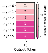
Layer 0 elevated the token ' 1' to be the 31st highest scored token in the hidden state it produced. Layers 1 and 2 kept increasing the ranking (to 7 then 5 respectively). All the following layers were sure this is the best token and gave it the top ranking spot.
Another visual perspective on the evolving hidden states is to re-examine the hidden states after selecting an output token to see how the hidden state after each layer ranked that token. This is one of the many perspectives explored by Nostalgebraist and the one we think is a great first approach. In the figure on the side, we can see the ranking (out of +50,0000 tokens in the model's vocabulary) of the token ' 1' where each row indicates a layer's output.
The same visualization can then be plotted for an entire generated sequence, where each column indicates a generation step (and its output token), and each row the ranking of the output token at each layer:
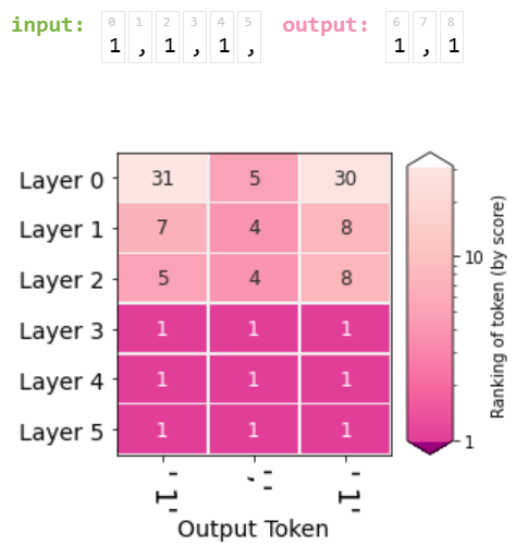
We can see that Layer 3 is the point at which the model started to be certain of the digit ' 1' as the output.
When the output is to be a comma, Layer 0 usually ranks the comma as 5.
When the output is to be a ' 1', Layer 0 is less certain, but still ranks the ' 1' token at 31 or 32. Notice that every output token is ranked #1 after Layer 5. That is the definition of greedy sampling -- the reason we selected this token is because it was ranked first.
Let us demonstrate this visualization by presenting the following input to GPT2-Large:
Visualizaing the evolution of the hidden states sheds light on how various layers contribute to generating this sequence as we can see in the following figure:
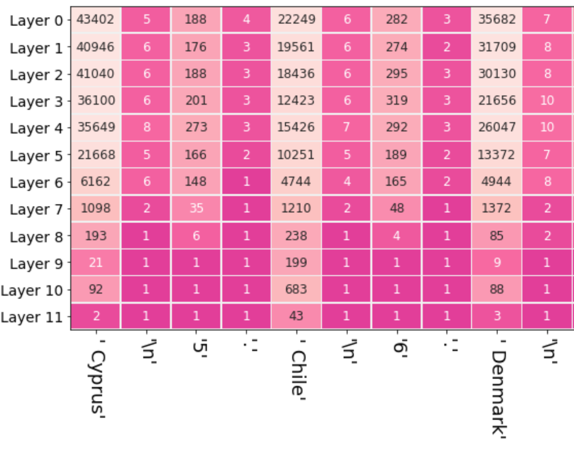
Click to open image in full resolution. The figure reveals:
- Columns of solid pink corresponding to newlines and periods. Starting from Layer #0 and onwards, the model is certain early on of these tokens, indicating Layer #0's awareness of certain syntactic properties (and that later layers raise no objections).
- Columns where country names are predicted are very bright at the top and it's up to the last five layers to really come up with the appropriate token.
- Columns tracking the incrementing number tend to be resolved at layer #9.
- The model erroneously lists Chile in the list, not a EU country. But notice that the ranking of that token is 43 -- indicating the error is better attributed to our token sampling method rather than to the model itself. In the case of all other countries they were correct and in the top 3.
- Aside from Chile, the rest of the countries are correct, but also follow the alphabetical order followed in the input sequence.
Rankings of Other Tokens
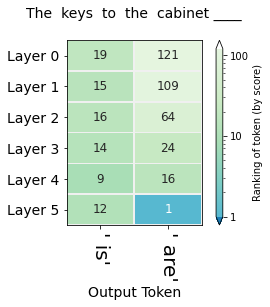
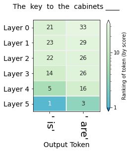
While the final output succeeds in assigning the correct number, the first five layers surprisingly fail at identifying the correct number (by giving " is" a higher ranking than " are", which is the correct answer). Examining attention or inner-layer saliency could reveal clues as to the reason.
We are not limited to watching the evolution of only one (the selected) token for a specific position. There are cases where we want to compare the rankings of multiple tokens in the same position regardless if the model selected them or not.
One such case is the number prediction task described by Linzen et al. which arises from the English language phenomenon of subject-verb agreement. In that task, we want to analyze the model's capacity to encode syntactic number (whether the subject we're addressing is singular or plural) and syntactic subjecthood (which subject in the sentence we're addressing).
Put simply, fill-in the blank. The only acceptable answers are 1) is 2) are:
The keys to the cabinet ______
To answer correctly, one has to first determine whether we're describing the keys (possible subject #1) or the cabinet (possible subject #2). Having decided it is the keys, the second determination would be whether it is singular or plural.
Contrast your answer for the first question with the following variation:
The key to the cabinets ______
The figures in this section visualize the hidden-state evolution of the tokens " is" and " are". The numbers in the cells are their ranking in the position of the blank (Both columns address the same position in the sequence, they're not subsequent positions as was the case in the previous visualization).
The first figure (showing the rankings for the sequence "The keys to the cabinet") raises the question of why do five layers fail the task and only the final layer sets the record straight. This is likely a similar effect to that observed in BERT of the final layer being the most task-specific. It is also worth investigating whether that capability of succeeding at the task is predominantly localized in Layer 5, or if the Layer is only the final expression in a circuit spanning multiple layers which is especially sensitive to subject-verb agreement.
Probing for bias
This method can shed light on questions of bias and where they might emerge in a model. The following figures, for example, probe for the model's gender expectation associated with different professions:
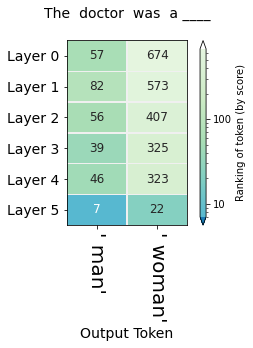
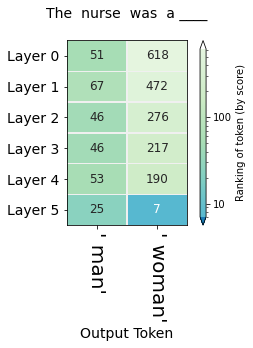
The first five layers all rank " man" higher than " woman" for both professions. For the nursing profession, the final layer decisively elevates " woman" to a higher ranking than " man".
More systemaic and nuanced examination of bias in contextualized word embeddings (another term for the vectors we've been referring to as "hidden states") can be found in .
Your turn!
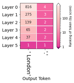
You can proceed to do your own experiments using Ecco and the three notebooks in this article: You can report issues you run into at the Ecco's Github page. Feel free to share any interesting findings at the Ecco Discussion board. I invite you again to read Interpreting GPT the Logit Lens and see the various ways the author examines such a visualization. I leave you with a small gallery of examples showcasing the responses of different models to different input prompts.Gallery
Model: DistilGPT2
Model: DistilGPT2


Model: DistilGPT2


Acknowledgements
This article was vastly improved thanks to feedback on earlier drafts provided by Abdullah Almaatouq, Anfal Alatawi, Fahd Alhazmi, Hadeel Al-Negheimish, Isabelle Augenstein, Jasmijn Bastings, Najwa Alghamdi, Pepa Atanasova, and Sebastian Gehrmann.
References
Citation
Alammar, J. (2021). Finding the Words to Say: Hidden State Visualizations for Language Models [Blog post]. Retrieved from https://jalammar.github.io/hidden-states/
BibTex:
@misc{alammar2021hiddenstates,
  title={Finding the Words to Say: Hidden State Visualizations for Language Models},
  author={Alammar, J},
  year={2021},
  url={https://jalammar.github.io/hidden-states/}
}

